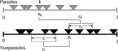
The niche model (Williams and Martinez 2000) is used to model the underlying predator–prey food web, and, as described below, parasites were added to the web. The niche model uses two fundamental parameters, connectance and species richness, and relies on a one-dimensional niche space or hierarchy. Species are given a random niche value n
i ∼ Uniform (0.1) in the hierarchy. Diets are assigned to each species independently by generating a center and a range as follows. Firstly, the feeding range is given by r
i = n
i
x
i where x is a random number drawn from a Beta distribution, with\documentclass[12pt]{minimal}
\usepackage{amsmath}
\usepackage{wasysym}
\usepackage{amsfonts}
\usepackage{amssymb}
\usepackage{amsbsy}
\usepackage{mathrsfs}
\usepackage{upgreek}
\setlength{\oddsidemargin}{-69pt}
\begin{document}$$ {x_i}\sim Beta\left( {\alpha = 1,\beta } \right) $$\end{document}. The distribution is chosen to obtain, on average, the desired connectance. Secondly, the centers of the feeding ranges are chosen randomly from species further down in the hierarchy, with \documentclass[12pt]{minimal}
\usepackage{amsmath}
\usepackage{wasysym}
\usepackage{amsfonts}
\usepackage{amssymb}
\usepackage{amsbsy}
\usepackage{mathrsfs}
\usepackage{upgreek}
\setlength{\oddsidemargin}{-69pt}
\begin{document}$$ {c_i}\sim {{Uniform}}\left( {{r_i}/2,{n_i}} \right) $$\end{document}. Once a feeding range is established for a given species, all species in that range become its prey. We add parasites to this model, by reversing the above rules as follows. First, a niche value ñ
k ∼ Uniform (0.1) is assigned to each parasite trophic species k. Parasites are also assigned feeding range sizes, but now these decrease as we move up the hierarchy, with \documentclass[12pt]{minimal}
\usepackage{amsmath}
\usepackage{wasysym}
\usepackage{amsfonts}
\usepackage{amssymb}
\usepackage{amsbsy}
\usepackage{mathrsfs}
\usepackage{upgreek}
\setlength{\oddsidemargin}{-69pt}
\begin{document}$$ {r_k} = \left( {1 - n} \right){y_k} $$\end{document}, where y
k is chosen from a Beta distribution properly chosen to obtain on average the observed connectance of the parasitic links. Parasites infect any nonparasite in their feeding range. However, now, the center of the parasites feeding range is drawn randomly from a position higher on the hierarchy, with \documentclass[12pt]{minimal}
\usepackage{amsmath}
\usepackage{wasysym}
\usepackage{amsfonts}
\usepackage{amssymb}
\usepackage{amsbsy}
\usepackage{mathrsfs}
\usepackage{upgreek}
\setlength{\oddsidemargin}{-69pt}
\begin{document}$$ {\tilde c_k}\sim {{Uniform}}\left( {{{\tilde n}_k},1 - {{\tilde r}_k}/2} \right) $$\end{document}. The larger feeding range is motivated by the concept that, if the hierarchy is related to size, parasites lower in the hierarchy, smaller in size, will typically have a larger potential feeding range, a larger set of hosts that can energetically support them. The parameters of the inverse niche model are: the number of parasites, the number of non-parasitic species, and the respective connectances of the parasite–nonparasite and nonparasite–nonparasite subwebs. Although for graphical convenience the niche axis is represented separately here for parasites and free-living species, this is in fact the same axis. Additional parameters could be introduced to restrict the parasitic niche space to map only onto a part of this segment

