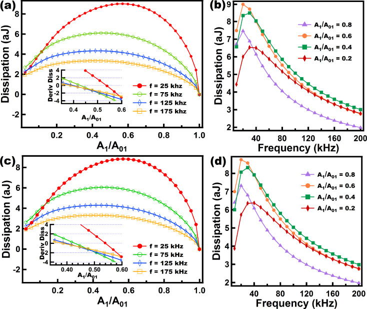
Figure 9.

(a) and (c) show dissipation vs amplitude setpoint (A₁/A₀₁) curves where each color coded line corresponds to a specific eigenfrequency, for the Wiechert and the SLS models, respectively. The insets in (a) and (c) show the slope of the curves in (a) and (c) plotted over a range near where the slopes cross the x-axis, in order to easily locate the maxima of the curves in (a) and (c). (b) and (d) show the behavior of dissipation as frequency increases, and each color coded line relates to a specific amplitude setpoint (A₁/A₀₁) for the Wiechert and the SLS models, respectively. The parameters for the cantilever dynamics were the same as in Figures 6 to 8. The sample parameters for (a) and (b) were: k_e = 10 N/m, k₁ = 7.5 N/m, k₂ = 7.5 N/m, c₁ = 0.5 × 10⁻⁵ N·s/m, and c₂ = 100.0 × 10⁻⁵ N·s/m. The sample parameters for (c) and (d) were: k_e = 17.5 N/m, k = 7.5 N/m, c = 0.5 × 10⁻⁵ N·s/m.