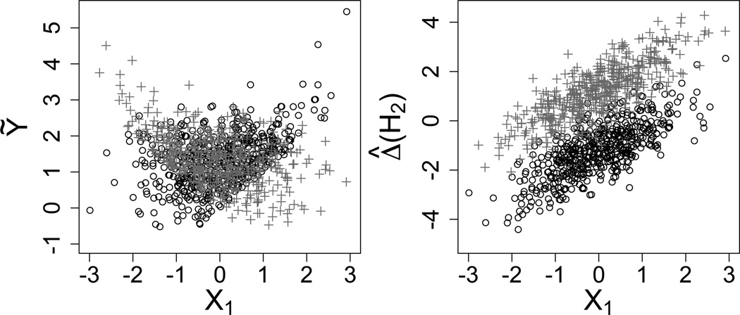
Fig. 1.
Scatterplots of Ỹ (left) and Δ̂(H2) (right) against X1 for A1 = −1 (black circles) and A1 = 1 (grey crosses) for 1, 000 random samples from the toy model. Step 2 of the Q-learning algorithm requires modeling the data in the left plot; note the nonlinearity and heteroscedasticity. Data in the right plot must be modeled for IQ-learning; note the common analysis of covariance structure.

