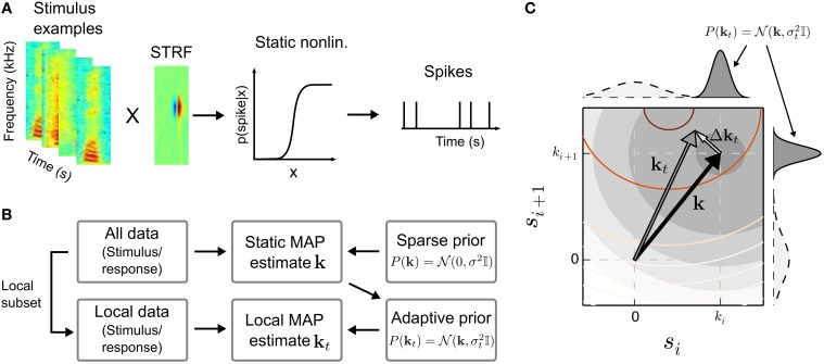
Figure 1.

Estimation of time-varying spectro-temporal receptive field (STRF) parameters in the linear-nonlinear model. (A) In the linear-nonlinear model, it is assumed that stimulus examples, represented here by spectro-temporal patches sampled from a speech spectrogram, are filtered by a linear filter k, the STRF. The output of the linear stage is transformed by a static non-linearity into a spike rate. In the generative model, a binary spike response is obtained by a subsequent inhomogeneous Poisson process. (B) A typical approach to infer the parameters of the model is the maximum a posteriori (MAP) estimate. The MAP allows to incorporate prior information, e.g., a prior that enforce sparseness by biasing STRF parameters toward zero by assuming a zero-mean Gaussian distribution of STRF parameters k. In the scenario of time-dependent neural processing, the MAP estimate obtained using all data, which constitutes the most probable static solution, may in turn be used as informative prior for a “local” (or time-dependent) MAP estimate k_t. Local evidence will result in deviations from the static STRF. (C) Illustration of the relation between static STRF k (black arrow) and local STRF k_t (gray arrow) in two stimulus dimensions s_i and s_{i + 1}. In case the likelihood (reddish contour lines) systematically deviates from the static prior (filled gray contours and gray marginal distributions), the maximum of the MAP estimate will be shifted by Δk_t resulting in a time-varying local STRF. The relatively flat marginal distributions of the sparse (zero-mean) Gaussian prior (dashed lines) indicate that the sparse solution would be dominated by the likelihood, which may be difficult to estimate for small sample sizes. For visualization purposes, the contour lines show likelihood and static prior on a logarithmic scale.