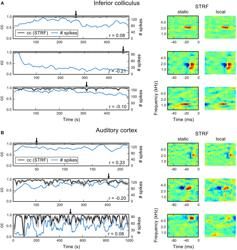
Figure 5.
Examples for time-dependent STRF analysis in auditory midbrain and cortex. For each part, we repeatedly estimated a local STRF using 90% of the data. To quantify the similarity between local and static STRFs, we used the correlation in terms of normalized subspace projection. Correlation values shown here are mean correlations across all 10 local bootstrap estimates. (A) Each row shows time-dependent correlations (denoted by cc) between local STRFs and static STRF (black line) and the corresponding number of spikes in the parts (blue line) for thee IC units. The gray shaded area indicates one standard deviation across the local bootstrap estimates. The arrows indicate the position of the local STRF example shown to the right, together with the static STRF. Numbers in the right lower corners indicate correlations between the cc trace and the number of spikes. (B) The same analysis for three A1 units. There is a considerable increase in fluctuations compared to IC examples. The local STRF examples primarily reveal changes in excitatory components at best frequency.

