Spike Train SIMilarity Space (SSIMS): a frame-work for single neuron and ensemble data analysis

Abstract

Increased emphasis on circuit level activity in the brain makes it necessary to have methods to visualize and evaluate large scale ensemble activity, beyond that revealed by raster-histograms or pairwise correlations. We present a method to evaluate the relative similarity of neural spiking patterns by combining spike train distance metrics with dimensionality reduction. Spike train distance metrics provide an estimate of similarity between activity patterns at multiple temporal resolutions. Vectors of pair-wise distances are used to represent the intrinsic relationships between multiple activity patterns at the level of single units or neuronal ensembles. Dimensionality reduction is then used to project the data into concise representations suitable for clustering analysis as well as exploratory visualization. Algorithm performance and robustness are evaluated using multielectrode ensemble activity data recorded in behaving primates. We demonstrate how Spike train SIMilarity Space (SSIMS) analysis captures the relationship between goal directions for an 8-directional reaching task and successfully segregates grasp types in a 3D grasping task in the absence of kinematic information. The algorithm enables exploration of virtually any type of neural spiking (time series) data, providing similarity-based clustering of neural activity states with minimal assumptions about potential information encoding models.

1 Introduction

Examining network function at larger and larger scales is now recognized as an important next step to understand key principles of brain network function and will require new methods to visualize and perform statistical comparisons between activity patterns observed over large sets of neurons (Alivisatos et al., 2013). Neurons often display complex response properties reflecting multiple behavioral and cognitive parameters (Sanes and Donoghue, 2000; Churchland et al., 2010; Rigotti et al., 2013). Characterizing these complex spiking patterns and describing how information from individual neurons is combined at the level of local ensembles and far-reaching networks is an ongoing challenge in neuroscience.

Many experiments involve recording ensemble activity (often in multiple areas) under various behavioral or cognitive conditions. Data analysis typically involves comparing binned firing rates across conditions using standard statistical tests, or fitting neuronal responses using models such as cosines or Gaussian distributions (Georgopoulos et al., 1982; Dushanova and Donoghue, 2010; Fluet et al., 2010; Li and DiCarlo, 2010; Pearce and Moran, 2012; Arimura et al., 2013). These methods often involve averaging across repetitions of a particular behavior, or otherwise summarizing neural activity patterns to a level where the ensemble properties are reduced to the equivalent of joint perievent histograms. This approach is prone to averaging out changes in a neural activity across trials. Furthermore, this level of data analysis and display becomes impractical as larger ensembles of neurons are recorded simultaneously. Methods to efficiently capture and display both spatial and temporal activity patterns in time series data are essential to both visualize and compare large-scale activity patterns and their relationship to behavior or activity in other brain areas.

At their core, most neural data analysis methods are interested in an assessment of similarity. For instance: when an experimental condition is changed, are neuronal spiking patterns similar or different, and what is the relative magnitude of the change? We have formulated a novel technique that provides a quantitative measure of similarity between neuronal firing patterns expressed on individual trials by either single neurons or ensembles. Our approach involves the combination of two key components: spike train distance metrics and dimensionality reduction.

Spike train metrics, as developed by Victor and Purpura, provide a measure of similarity between pairs of spike trains by calculating the most direct way to transform one spike train it another by inserting, deleting, or moving spikes such that both patterns coincide (Victor and Purpura, 1996, 1997; Victor, 2005). Adding up a cost assigned to each of these operations provides quantitative measure of the similarity between activity patterns. The use of spike train metrics makes it possible to analyze long time periods (on the order of seconds) while preserving structure inherent in millisecond scale spike timing. Changing the cost assigned to temporal shifts offers the opportunity to examine neural activity at multiple temporal resolutions.

Dimensionality reduction is often accomplished by model fitting, such as by fitting tuning functions. When the model relating neural observations with the behavior/stimulus is unknown, model-free methods such as principal component analysis can be used to gain insight into the relationship. Here we employ t-Distributed Stochastic Neighbor Embedding (t-SNE) (van der Maaten and Hinton, 2008) to project the high-dimensional space defined by pair-wise spike train distances into a low-dimensional representation which not only facilitates visualization, but also improves pattern discrimination. This method is well suited to this type of analysis because it is based on pair-wise similarity estimates and explicitly seeks to preserve the structure within local neighborhoods (in this case, clusters of individual trials with similar activity patterns).

The proposed algorithm transforms neural data to produce a low dimensional ‘Spike train SIMilarity Space’ (SSIMS) that represents the relationships between activity patterns generated on individual trials. In the SSIMS projection, similar neural activity patterns cluster together, while increasingly different activity patterns are projected further apart. The degree of similarity between activity patterns of interest can be clearly visualized and quantified. Furthermore, SSIMS projections can be used to evaluate the similarity between training data and new samples, providing a direct basis for pattern classification (decoding). The goal of this report is to describe the method, illustrate its implementation, and examine the strengths and limitations of the approach.

We tested and validated the SSIMS algorithm using the activity of multiple single neurons recorded simultaneously in primate primary motor and premotor cortex, successfully separating neural activity patterns reflecting the behaviors performed in both a planar center-out reaching task and a 3D reaching and grasping task. The method provides a useful framework for data analysis and visualization well suited to the study of large neuronal ensembles engaged in complex behaviors.

2 Description of the SSIMS algorithm

The goal of the SSIMS algorithm is to numerically quantify the similarity between multiple neural activity patterns. We define the ‘state’ of a given ensemble of neurons over a specific time period as the precise timing of each spike fired by each neuron; for example, if the patterns of activity for all neurons during two different time periods can be perfectly aligned, the corresponding ensemble states are considered to be identical.

The algorithm consists of two parts. First, pair-wise similarity estimates between spike trains are obtained using the distance metric proposed by Victor and Purpura, spikes necessary to transform one spike train into another (Victor and Purpura, 1996). This process results in a high-dimensional space representing pair-wise similarities between the sampled ensemble firing patterns (for example, a series of trials in a behavioral task). In order to facilitate statistical analysis and data visualization, the second part of the algorithm refines the high-dimensional space defined in terms of these pair-wise distances using the t-SNE dimensionality reduction technique developed by van der Maaten and Hinton (2008). Within SSIMS projections, distances between points denote the degree of similarity between the ensemble firing patterns (putative network ‘states’) they represent; clustering of points that correlate with experimental labels (such as behavioral conditions) allows an unbiased assessment of the relationship between neural states within the context of the experimental variables.

2.1 Measuring the similarity between two spike trains

Victor and Purpura introduced cost-based metrics designed to evaluate the similarity between spike trains (Victor and Purpura, 1996). A given spike train, A, can be transformed into second spike train, B, using three basic operations: the addition of a spike, the deletion of a spike, or the shifting of a spike in time. Each of these operations is assigned a ‘cost’; the distance between the two spike trains is defined as the (minimum) summed cost of the operations needed to transform one into the other. The cost of spike insertion or deletion is set to 1, while the cost of shifting a spike in time is set to be proportional to the length of time the spike is to be shifted. This last value is defined using a parameter q, with the cost of shifting a spike being qΔt. Note that displacing a spike by a time interval 1/q has a cost equivalent to deleting it. In this way, the value of q is related to the temporal precision of the presumed spike code, in the sense that it determines how far a spike can be moved in time while still considering it to be the ‘same’ spike (that is, without having to resort to removing it). Setting q = 0 makes the timing of a spike irrelevant, reducing all shifting costs to zero. In this case the distance function is effectively reduced to a difference in spike counts. In this way, this method can be used to probe possible values for the temporal resolution of neural data, from millisecond timing to pure rate codes.

2.2 Creating a similarity space based on pair-wise distances

Let us consider a set of n neurons, whose activities are simultaneously recorded over a set of m trials (with each neuron generating a spike train during each trial). Let D_spike(A, B) denote the spike train distance metric as defined by Victor and Purpura (1996): the minimum cost of transforming spike train A into spike train B. Let S_i,j represent the spike train recorded from neuron j during the i-th trial. Let the pairwise similarity vector for spike train S_i,j be defined as:

$${\mathrm{d}}_{\text{pw}}(S_{i,j})=(D_{\text{spike}}(S_{i,j},S_{1,j}),D_{\text{spike}}(S_{i,j},S_{2,j}),\dots ,D_{\text{spike}}(S_{i,j},S_{m,j}))$$

Thus, each spike train from a single neuron can be mapped to a m-dimensional space by representing it as a vector of pair-wise distances to the other spike trains fired by the same neuron. An ensemble pair-wise similarity vector for trial i is formed by concatenating the d_pw vectors of the n neurons:

$${\mathrm{D}}_i^{\text{ensemble}}={({\mathrm{d}}_{\text{pw}}(S_{i,1}),\dots ,{\mathrm{d}}_{\text{pw}}(S_{i,n}))}^T$$

Thus, the neural activity for each individual trial is represented by a 1 × mn dimensional vector which includes m similarity measurements for each neuron. When the vectors for each of the m trials are combined into a matrix for an ensemble of n neurons, the result is an m × mn matrix we refer to as D^ensemble which constitutes a relational embedding of the entire data set. Note that in this formulation the information obtained from a given neuron is represented in a separate subset of dimensions of the matrix D^ensemble (instead of summing cost metrics across neurons to 155 obtain a single measure of ensemble similarity). The next part of the algorithm seeks to project D^ensemble into a lower dimensional space.

2.3 Dimensionality reduction with t-SNE

As we will show later, it is possible to create low dimensional representations based on neural ensemble pairwise similarity data that increase the accuracy of pattern classification, preserving nearest-neighbor relationships without information loss. The SSIMS method uses the t-SNE algorithm, which is particularly well suited to our approach because it explicitly models the local neighborhood around each point using pair-wise similarity measures (van der Maaten and Hinton, 2008). The general intuition for the algorithm is as follows: given a particular data point in a high dimensional space, one is interested in picking another point that is similar; that is, another point that is in the same ‘local neighborhood’. However, instead of deterministically picking a single closest point, one selects the local neighbor in a stochastic manner, according to a probability (making the probability of selecting points that are close together high, and those that are very far apart low). The set of resulting conditional probabilities (given point A, what is the likelihood that point B is a local neighbor?) effectively represents similarity between data points. The local neighborhoods around each point are modeled as t-distributions. Rather than using a fixed value for the width of the distribution (σ) across the entire space, the algorithm uses multiple values of σ determined by the data density in the local neighborhood around each point. The span of each of these local neighborhoods is determined by the ‘perplexity’ parameter setting of the algorithm, which determines effective number of points to include. Note that if a given dataset contains a dense cluster and a sparse cluster, the size of the local neighborhoods in the sparse cluster will be larger than those in the dense cluster. This dynamic adaptation of local neighborhood size serves to mitigate the ‘crowding problem’, which arises when attempting to separate clusters with different densities using a single fixed neighborhood size (which potentially leads to over-sampling the dense cluster or under-sampling the sparse one). Probability distributions describing local neighborhoods are modeled using pair-wise distances, which can be evaluated regardless of the dimensionality of the space. It is therefore possible to compare the similarity of the local neighborhoods for high and low dimensional versions of a given dataset. By minimizing the difference between the two sets of conditional probabilities, the local neighborhood structure is preserved in the low-dimensional mapping.

In order to reduce computational complexity, we perform a preliminary round of dimensionality reduction using principal component analysis (PCA) to project the D^ensamble matrix into a 100-dimensional space. The t-SNE algorithm then refines the resulting linear transform by minimizing the Kullback-Leibler divergence between local neighborhood probability functions for this starting point and progressively lower dimensional spaces via gradient descent. Using the terminology from the previous section, the final output of the t-SNE algorithm is a mn × d matrix (the t-SNE transform), which projects the m × mn D^ensemble matrix into the desired d dimensional space (where n is the number of neurons and m is the number of spike trains).

2.4 Software, Hardware, and processing time

Calculations were performed using MatLab on a Mac workstation with a 2.93 GHz quad-core Intel Xeon processor and 12GB of RAM. Using this hardware, producing a two-dimensional representation of neural activity for ~100 trials based on the firing patterns of ~100 neurons over one second took, on average, five seconds (including the processing time required to calculate all pair-wise distances between spike trains starting from a list of spike timestamps for each neuron). The source code used for data analysis will be made freely available for non-commercial use at the Donoghue lab website. The algorithm could be modified for near real-time discrete classification in the following manner: First, a training dataset with exemplars in each desired category would be collected. After calculating all pair-wise distances the t-SNE transform would be calculated as described above (taking only a few seconds after data has been collected). The resulting SSIMS space would provide a relational reference frame to interpret new incoming data. Note that once the t-SNE transform is calculated, projecting new data samples into the resulting SSIMS representation would only take a fraction of the time since the gradient descent part of t-SNE is no longer required. It would still be necessary to calculate pair wise distances for new data samples, but this would involve only m operations per neuron in order to project a new trial into the original SSIMS representation (as opposed to the n × m² operations needed to generate the initial embedding). Furthermore, pair-wise distance calculation is well suited to parallel computing and could be further optimized using multi-threading or specialized hardware. Parallel streams could also be used to independently update the t-SNE transform incorporating new data, providing updated SSIMS embeddings on demand. Overall, the limiting factor on processing time would be the duration of the time window to be analyzed, which would depend on the precise nature of the spiking patterns being classified. The results presented in the following sections suggest that an 8-way classification with >95% accuracy could be accomplished in under one second.

3 SSIMS algorithm validation using primate cortical ensemble activity

Performance of the algorithm was evaluated using cortical ensemble activity recorded in rhesus macaques (Macaca mulatta) using 96 channel chronically implanted micro-electrode arrays. Details of the implantation procedure are described in Suner et al. (2005) and Barrese et al. (2013). All procedures were approved by the Brown University Institutional Animal Care and Use Committee. Two datasets were used to illustrate the implementation of the method and its properties. The first consisted of neural data recorded in primary motor cortex (MI) from a monkey performing a planar center-out reaching task. The second dataset consisted of neural data recorded in ventral premotor cortex (PMv) from a monkey performing a naturalistic reaching and grasping task that involved intercepting and holding moving objects in a 3D workspace.

3.1 Electrophysiological Recording

During each recording session, signals from up to 96 electrodes were amplified (gain 5000), bandpass filtered between 0.3 kHz and 7.5 kHz, and recorded digitally at 30 kHz per channel using a Cerebus acquisition system (Blackrock Microsystems, Salt Lake City, UT). Waveforms were defined in 1.6 ms data windows starting 0.33 ms before the voltage crossed a threshold of at least −4.5 times the channel root mean square variance. These waveforms were then sorted using a density clustering algorithm (Vargas-Irwin and Donoghue, 2007), the results of which were reviewed using Offline Sorter (Plexon, Dallas TX) to eliminate any putative units with multiunit signals (defined by interspike intervals (ISI) <1 ms) or signal to noise ratios (SNR) less than 1.5.

3.2 Center-out (COUT) task

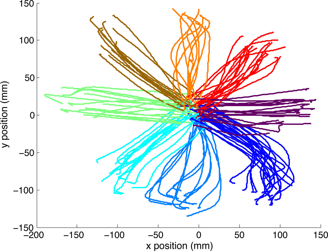
One monkey was operantly trained to move a cursor that matched the monkey’s hand location to targets projected onto a horizontal reflective surface in front of the monkey. The monkey sat in a primate chair with the right arm placed on individualized, cushioned arm troughs secured to links of a two-joint exoskeletal robotic arm (KINARM system; BKIN technologies, Kingston ON, Canada; Scott, 1999) underneath an image projection surface that reflected a computer monitor display. The shoulder joint was abducted 85° so that shoulder and elbow movements were made in an approximately horizontal plane. The shoulder and elbow joint angles were digitized at 500 Hz by the motor encoders at the joints of the robotic arm. The x and y positions of the hand were computed using the standard forward kinematic equations and sampled at 200 Hz. For more details on the experimental setup using the KINARM exoskeleton, refer to Rao and Donoghue (2014). Neural data was simultaneously recorded from a chronically implanted microelectrode array in the upper limb area of primary motor cortex. To initiate a trial, the monkey was trained to acquire a target in the center of the workspace. A visual cue was used to signal movement direction during an instructed delay (with duration 1 – 1.6 s) to one of eight radially distributed targets on a screen. At the end of the instructed delay period, the central target was extinguished, instructing the monkey to reach towards the previously cued target. Movement onset was defined as the time when the cursor left the central target. The trajectories for each of the eight movement directions are shown in Figure 1.

Figure 1. Center out task kinematics.

The trajectories show the position of the tip of the index finger as the monkey performs a center-out motion to 8 peripheral targets (labeled from 0 to 315°). The trajectories shown were taken from a 1-second time window starting 100ms before movement onset (corresponding to the main time period used for neural data analysis).

3.3 Center-out task: Single neuron properties

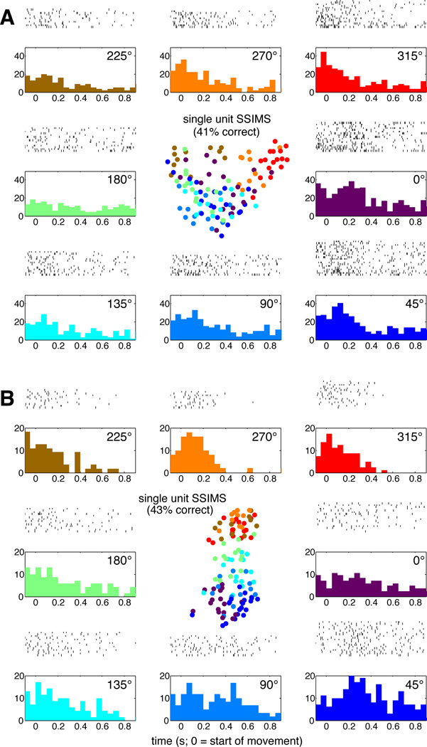
We first validated the algorithm by generating SSIMS projections for individual neurons over a time window of one second starting 100 ms before movement onset (using q = 10, such that 1/q = 100 ms, SSIMS dimensionality = 2 and t-SNE perplexity = 30). Figure 2 shows two samples of single-neuron SSIMS projections, as well as traditional raster plots. While the raster plots clearly convey the changes in the mean firing rate averaged across trials, it is difficult to discriminate the variability in the firing patterns for each movement direction.

Figure 2. Single neuron SSIMS in the Center-out task.

A. The outer plots show traditional raster-histograms (50 ms bins) for each of the 8 movement directions (radially arranged to represent their relative position on the workspace as shown in Fig. 1). The central plot shows the SSIMS representation for the same data. Each trial shown in the raster plots corresponds to a single point in the SSIMS representation. Color coding is used to match SSIMS points with the corresponding movement directions. A KNN classifier operating on the SSIMS representation of this single unit was capable of correctly predicting the direction of 41% of the trials (see main text for details). B. Similar comparison with a second neuron.

The SSIMS plot represents the spike train for each trial as a single point. This representation shows that the firing patterns for the neuron in Figure 2A are more tightly clustered for the 315° direction (representing a greater degree of similarity). Further-more, the figure reveals that the firing patterns are most similar between 315° and 270° reaches. It is also possible to identify individual 0° trials where this neuron fires in a manner very similar to 315° trials. Note that, in this case, the direction presenting the most tightly clustered firing pattern is not the direction of with the highest firing rate (0°), which would be labeled as the ‘preferred direction’ if firing rates were parameterized with a standard cosine fit. Also note that the most tightly clustered pattern does not correspond to the direction with lowest firing rate, as might be expected if a Poisson noise model is assumed. The neuron shown in Figure 2B is also difficult to describe in terms of standard models, since the timing of the peak in firing rate appears to change as a function of direction. The preferred direction for this neuron would there-fore change as a function of time if it were evaluated using short time windows. The SSIMS algorithm is able to display spiking patterns over a time frame encompassing the entire movement. The resulting plot clearly shows that the greatest difference in spiking patterns exists between 225°, 270°, and 315° reaches compared to 0° and 45°, with the remaining directions roughly in the middle. This layout reflects the relationships between the neural activity patterns observed across reach directions that would be difficult to capture using standard tuning functions.

We tested for significant direction-related clustering at the level of single neurons by comparing the distribution of SSIMS distances within and between directions using a Kruskal-Wallis test. Neurons were identified as being directionally selective when the median SSIMS distance was smaller between trials in the same direction compared to trials in different directions. A 10D SSIMS projection was used for this operation, to encompass high dimensional features not visible in 2D projections. Eighty-three out of 103 recorded neurons (~81%) were determined to be directionally selective using this method (Kruskall-Wallis p < 0.001). For comparison, a Kruskall-Wallis test performed directly on the firing rates for the same time period only produced p values < 0.001 for 70% of the neurons.

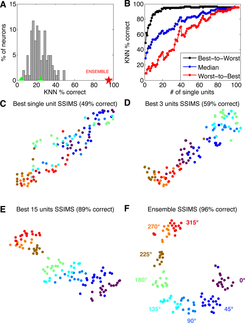
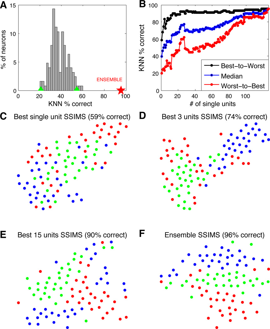
The magnitude of directional selectivity for individual neurons was evaluated using a nearest neighbor (NN) classifier implemented using leave-one-out cross validation. Each trial was classified based on the direction of the nearest neighbor in the 10D SSIMS projection. The percent of correctly classified trials was used as a measure of directional information for a given neuron. The distribution of average single-neuron classification results is shown in Figure 3A. These values were used to rank the neurons from most to least informative.

Figure 3. Center out task: From single neurons to ensembles.

A. Single neuron performance in 8-direction classification (10D SSIMS, NN classification using data from individual neurons separately). Classification accuracy using the combined data from all neurons is highlighted with a red star for comparison. Green triangles denote the 95% confidence interval of the chance distribution (calculated over 10,000 random shuffles of the trial labels). B. Classification performance as a function of ensemble size (10D SSIMS). Neurons were ranked according to single-unit NN results and added to the decoding ensemble from best to worst (black) or worst to best (red). The median value between these two extremes is shown in blue, representing the expected trend for randomly chosen neurons. C–F. SSIMS projections for various ensemble sizes (2D SSIMS). Color coding denotes reach direction using the same conventions as figure 2 (directions are also highlighted in panel F).

Ensemble decoding was performed using two different strategies: neurons were added to the decoding ensemble from most to least informative (providing an approximate upper bound for classification) or in the reverse order (to generate an approximate lower bound). Classification accuracy (using a KNN classifier with k = 1, implemented with leave-one-out cross validation) is shown as a function of ensemble size for both curves in Figure 3B. Figure 3C–F displays the relationship between ensemble activity in each of the 8 movement directions as neurons are progressively added. Although classification was performed in a 10-dimensional space, the SSIMS algorithm was used to project the data down to two dimensions for ease of visualization (classification using 2 or 3D SSIMS produced similar results on average, but with greater variability). Note that when the entire ensemble is used, the shape of the clusters matches the directions of movement, generating a circular pattern where clusters are arranged from 0 to 315 degrees. This structure emerges solely from the relationship between the firing patterns, since clustering is performed without any information about the movement direction associated with each trial. Color coding is added after the fact for visualization; this information about the task is not utilized by the SSIMS algorithm.

3.4 Free Reach-to-Grasp (FRG) task

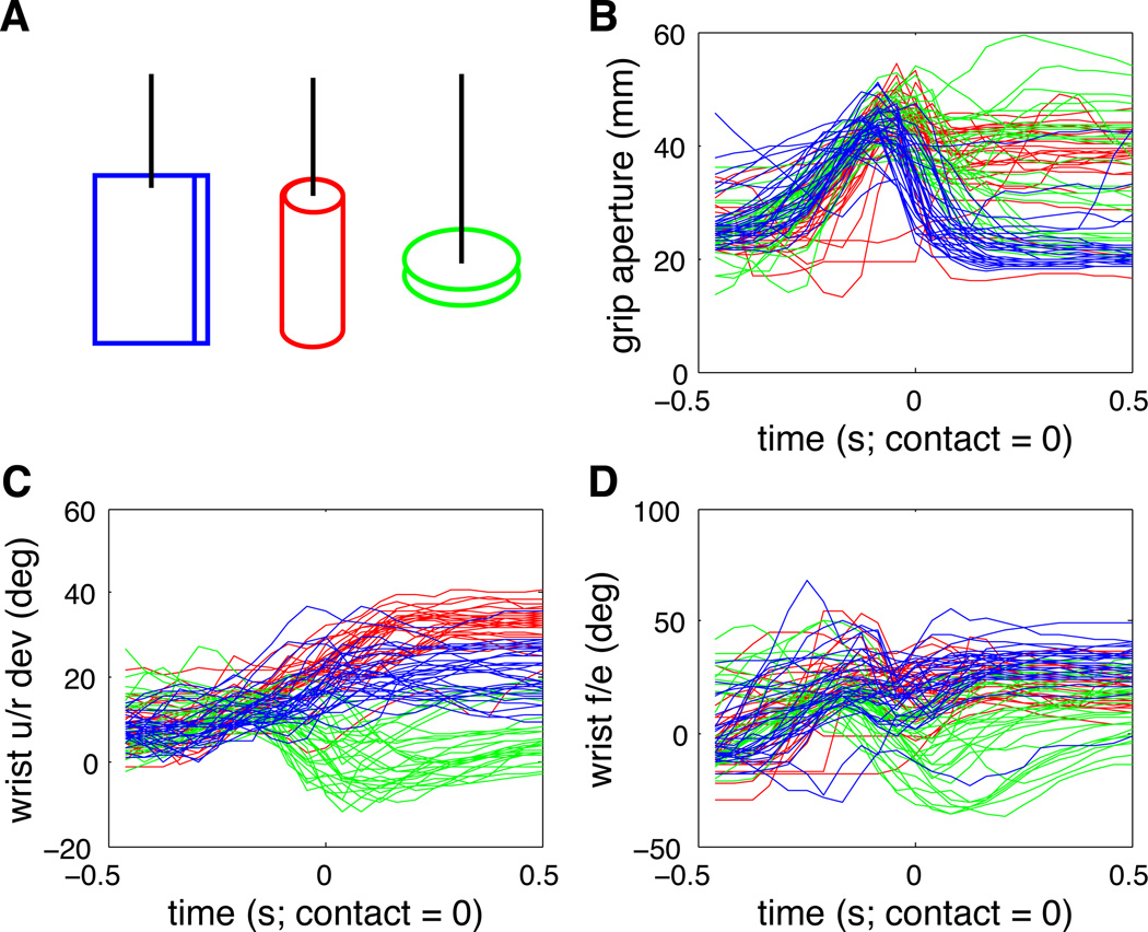
In the Free Reach-to-Grasp (FRG) task, monkeys were required to intercept and hold objects swinging at the end of a string (Figure 4A). After successfully holding an object for one second, they received a juice reward and were required to release the object to initiate a new trial. The objects were presented at different positions and speeds. Three different objects were used (one at a time) in order to elicit different grasping strategies. The first object was a vertical plate 10 cm high by 7 cm wide by 0.3 cm thick. The second object was a vertical 18 cm long cylinder with a 2.5 cm diameter. The third object was a horizontal disk 7.5 cm in diameter and 0.3 cm thick. The monkey’s movements were measured using an optical motion capture system (Vicon Motion Systems Ltd. UK) to track reflective markers attached to the skin as described in Vargas-Irwin et al. (2010). For this dataset we measured grip aperture (the distance between markers placed on the distal interphalangeal joint of the index finger and thumb) as well as wrist flexion/extension and ulnar/radial deviation subsampled at 24 Hz (Figure 4B–D). Object contact was detected using capacitative switches built into the objects.

Figure 4. Free Reach-to-Grasp task kinematics.

A. Diagram of the target objects (not to scale). Each one was presented at the end of a string moving through points in the workspace. B–D. Hand kinematics measured using optical motion capture spanning one second centered on object contact. Color coding matches object color in panel A (blue = vertical plate, red = cylinder, green = disk). Grip aperture was measured as the distance between markers placed on the distal-most joints of the index and thumb. Wrist u/r dev = ulnar/radial deviation; f/e = flexion/extension.

3.5 Free Reach-to-Grasp task: Single neuron properties

Spike trains, one second in duration, were recorded from PMv and centered on each successful object contact event (where the grip was maintained for at least one second). Neural activity and kinematics were collected for a total of 90 trials (30 with each object). SSIMS projections for classification were derived from the neural data using q = 10, such that 1/q = 100 ms, SSIMS dimensionality = 10 and t-SNE perplexity = 30.

Single unit properties were tested using the same strategy employed in the center-out task. We tested for significant grasping-related clustering by comparing the distribution of SSIMS distances within and between categories using a Kruskal-Wallis test. Neurons were identified as being object selective when the median SSIMS distance was smaller between trials with the same object compared to trials with different objects. Forty-seven out of 126 recorded neurons (~37%) were determined to be selective using this method (Kruskall-Wallis p < 0.001). For comparison, a Kruskall-Wallis test performed directly on the firing rates for the same time period only produced p values < 0.001 for 19% of the neurons. As with the center-out data, the magnitude of directional selectivity for individual neurons was evaluated using a nearest neighbor (NN) classifier implemented using leave-one-out cross validation. Single-unit classification results are summarized in Figure 5A. These values were used to rank the neurons from most to least informative. Classification accuracy (using a NN classifier) is shown as a function of ensemble size in Figure 5B (for neurons added from best to worst, or in the inverse order).

Figure 5. FRG task: from single neurons to ensembles.

A. Single neuron performance in 3-object classification (10D SSIMS, NN classification using data from individual neurons separately). Classification accuracy using the combined data from all neurons is highlighted with a red star for comparison. Green triangles denote the 95% confidence interval of the chance distribution (calculated over 10,000 random shuffles of the trial labels). B. Classification performance as a function of ensemble size (10D SSIMS). Neurons were ranked according to single-unit NN results and added to the decoding ensemble from best to worst (black) or worst to best (red). The median value between these two extremes is shown in blue, representing the expected trend for randomly chosen neurons C–F. SSIMS projections for various ensemble sizes (2D SSIMS).Color denotes the object being grasped (blue = vertical plate, red = cylinder, green = disk).

Figure 5C–F displays the relationship between ensemble activity patterns associated with the three objects as neurons are progressively added to the ensemble (for ease of visualization 2D SSIMS projections are shown). The target object clearly emerges as the dominant feature in the SSIMS projections; this can bee seen in the post-hoc color coding. Note that this result does not imply that other kinds of information – such as hand position – are not represented in the neural data. With greater numbers of neurons cluster separation and classification performance gradually increase. A NN classifier (implemented with leave-one-out cross validation) applied to the full ensemble SSIMS projections correctly identified the target object in ~96% of the trials, exceeding results obtained using a similar classifier applied directly on all kinematic measurements shown in Figure 4 spanning the same time duration (89% correct). Measuring additional kinematics and or dynamics could potentially narrow the gap between neural and kinematic classification. However, our results demonstrate that the SSIMS algorithm is capable of capturing grasp-related activity patterns with fidelity on par with detailed kinematic measurements. The method can successfully discriminate activity patterns in complex tasks involving many interacting degrees of freedom, and is therefore a potentially useful tool for the analysis of high-dimensional motor, sensory, or cognitive neural responses.

3.6 Comparison with other methods

The SSIMS algorithm combines spike train similarity metrics with t-SNE in order to generate low-dimensional representations of neural spiking data. It is possible to generate similar outputs by combining different pre-processing and dimensionality reduction techniques. In order to examine the contributions different approaches, we tested two pre-processing methods with three dimensionality reduction algorithms. The preprocessing methods analyzed were spike train similarity metrics (SIM) and binned spike counts (SC), while the dimensionality reduction algorithms were t-SNE, multidimensional scaling (MDS), and principal component analysis (PCA). Each combination was evaluated using a NN classifier (as described in previous sections) for both the COUT and FRG task data. Each pre-processing method was evaluated at two temporal accuracy settings (100msec bins, equivalent to 1/q = 100msec, and 10msec bins, equivalent to 1/q = 10msec). In all comparisons one second of neural data was used. Each dimensionality reduction algorithm was used to generate a 10D space (well-suited for classification) as well as a 2D space (for ease of visualization). Additionally, we ran the NN classifier on data without the benefit of dimensionality reduction as a baseline comparison. Results are summarized in Table 1.

Table 1. Pairing neural data pre-processing and dimensionality reduction strategies.

Classification results obtained using a NN classifier on data processed using different combinations of algorithms. Column headings denote the dimensionality reduction algorithm: principal component analysis (PCA), multidimensional scaling (MDS), t-distributed stochastic neighbor embedding (t-SNE), or ‘RAW’ when no dimensionality reduction was performed. Each column heading also lists the data pre-processing method: spike counts (COUNTS), or spike train similarity metrics (SIM). The highest classification values for each task, dimensionality, and temporal accuracy setting (rows) are highlighted. A. Results for temporal accuracy of 100msec (1/q = 100msec for SIM, bin size = 100msec. for COUNTS) B. Results for temporal accuracy of 10msec. In 7 out of 8 combinations of dataset, temporal accuracy setting, and dimensionality (table rows) the SSIMS algorithm (t-SNE + SIM) outperformed or matched the classification accuracy obtained using any of the other methods evaluated.

		RAW COUNTS	RAW SIM.		PCA COUNTS	PCA SIM.	MDS COUNTS	MDS SIM.	t-SNE COUNTS	SSIMS
A	FRG (100ms)	79%	89%	10D	76%	91%	73%	91%	83%	96%*
				2D	40%	29%	42%	58%	70%	87%*
	COUT (100ms)	91%	96%*	10D	96%*	95%	95%	95%	96%*	96%*
				2D	60%	57%	86%	86%	98%*	97%
B	FRG (10ms)	40%	91%	10D	57%	90%	51%	91%	62%	92%*
				2D	36%	42%	42%	50%	44%	88%*
	COUT (10ms)	19%	92%	10D	84%	95%	56%	95%	54%	96%*
				2D	55%	39%	89%	86%	68%	96%*

Across all of the comparisons evaluated, methods using spike counts produced, on average, 67% correct classification (s.dev = 20), while methods based on spike train similarity averaged 80%. Methods including PCA averaged 65% (s.dev = 24), while the average for MDS was 74% (s.dev = 20), and the average for t-SNE was 83% (s.dev = 17). For any given task, dimensionality, and temporal accuracy, the combination of techniques used in the SSIMS algorithm (SIM + t-SNE) produced the highest accuracy observed, with the exception of COUT, 2D, and 100msec, where it was 1% below t-SNE + spike counts.

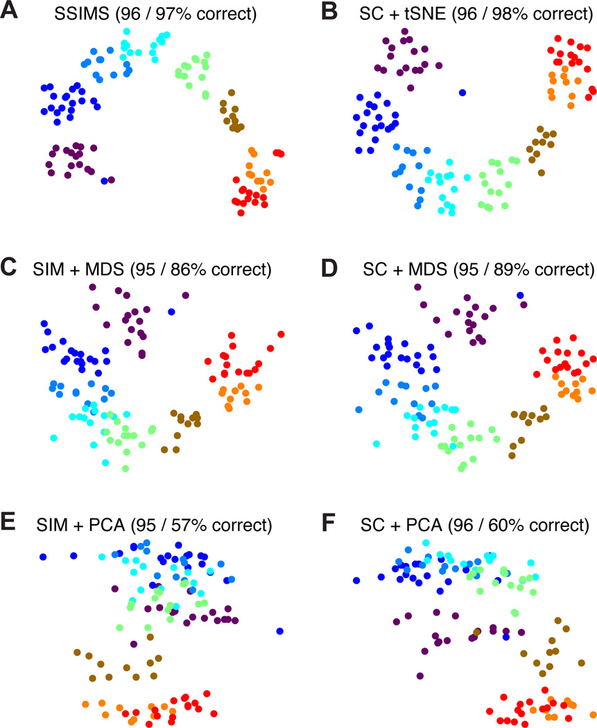
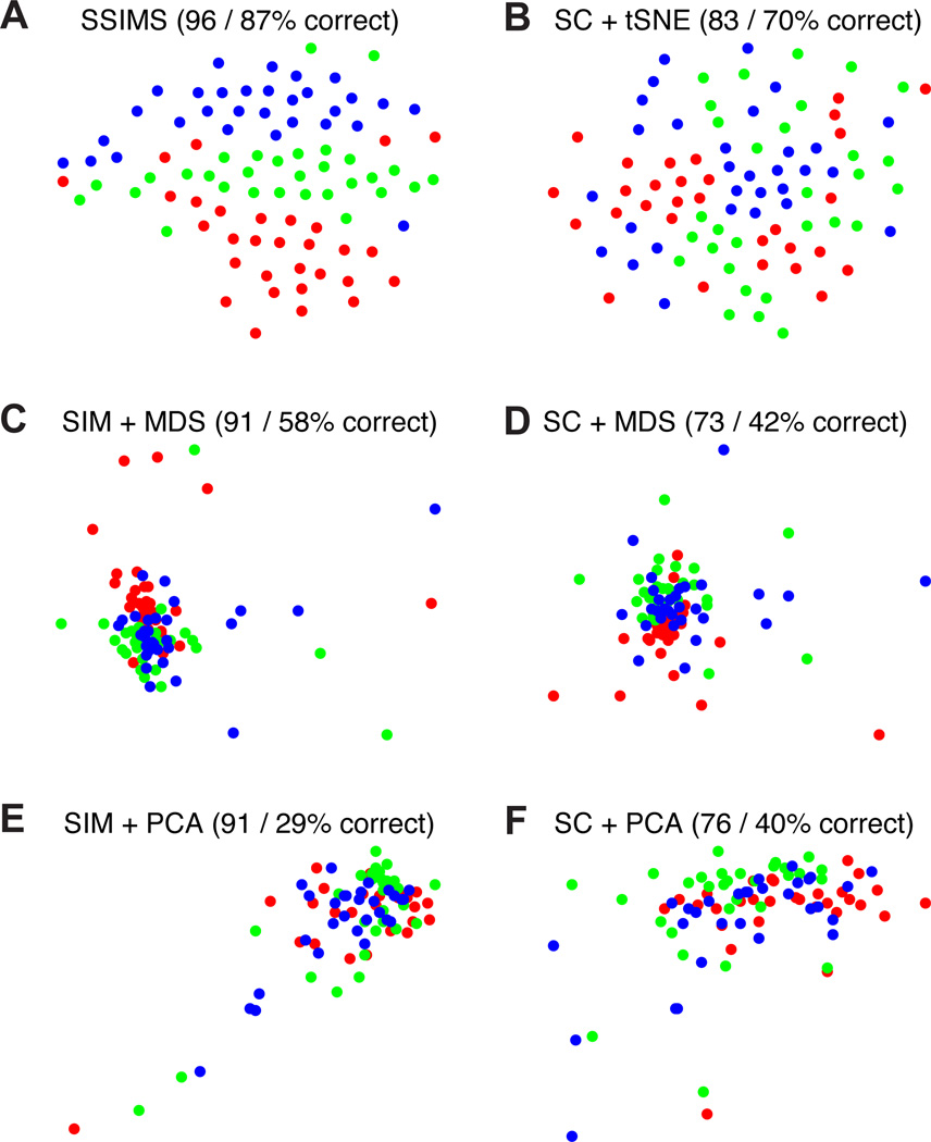
Overall, similarity metrics tended to outperform spike counts and produce representations which were more stable across different dimensionality settings. The largest differences between dimensionality reduction algorithms were observed in the 2D spaces, where t-SNE was clearly superior. For 10D spaces the performance of different algorithms was relatively similar (especially when using spike train similarity as a preprocessing step). This pattern suggests that even for cases where discrete classification accuracy for MDS and t-SNE is roughly equivalent, t-SNE consistently produces more informative 2D plots for visualization purposes. Samples of 2D plots produced using different methods are shown in Figs. 6 and 7. Note that PCA fails to capture the circular arrangement of targets in the COUT task (Fig. 6 ). This pattern is revealed by MDS, but the clusters tend to be more diffuse than those obtained using t-SNE. The differences are more pronounced for the FRG task, where only the full SSIMS algorithm shows a clear recognizable pattern in 2D (Fig. 7).

Figure 6. Neural data visualization: COUT task.

Top row shows results using tSNE for the dimensionality reduction step (A,B), middle row represents MDS (C,D) and bottom row PCA (E,F). Left column shows results for methods using spike train similarity as a pre-processing step (A,C,E), right column shows results for methods based on spike counts (B,D,F).

Figure 7. Neural data visualization: FRG task.

Top row shows results using tSNE for the dimensionality reduction step (A,B), middle row represents MDS (C,D) and bottom row PCA (E,F). Left column shows results for methods using spike train similarity as a pre-processing step (A,C,E), right column shows results for methods based on spike counts (B,D,F).

3.7 Effects of Parameter Setting on SSIMS algorithm performance

We tested the performance of the SSIMS algorithm under a range of parameter settings spanning a range of spike train durations, temporal offsets, dimensionality, temporal resolution (q values), and perplexity. Algorithm performance was evaluated based on classification accuracy of either reaching direction in the COUT task or target object for grasping in the FRG task. In both cases, a nearest neighbor classifier with leave-one-out cross validation was applied as previously described.

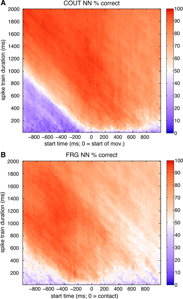
For both of the tasks examined, accurate pattern classification (greater than 85% correct) was observed for a wide range of time windows (Figure 8). For the COUT task, the most informative time period for direction classification was around the time of start of movement. In the FRG task, the most informative period for grip classification was roughly 500 ms before contact with the object, coinciding with the transport phase that includes hand pre-shaping. The duration of the time window analyzed had a relatively small effect on performance. During the most informative time periods, time windows of as short as 200 ms were sufficient for accurate classification. Extending the time window by an order of magnitude (up to 2 s) did not adversely affect performance. These results show that the SSIMS method is suitable for exploring neural data at a broad range of time scales.

Figure 8. Effect of spike train duration and temporal offset on SSIMS.

A. Effects of temporal offset and spike train duration on COUT direction classification. The abscissa is the start time for the window used to generate the SSIMS projection (centered around start of movement; negative values are before the onset of movement). The ordinate varies the length of the time window. These results were obtained holding q = 10 (corresponding to a temporal precision of 0.1 s), perplexity = 30, and SSIMS dimensionality = 10. B. Effects of temporal offset and spike train duration on FRG grip classification (same conventions as A).

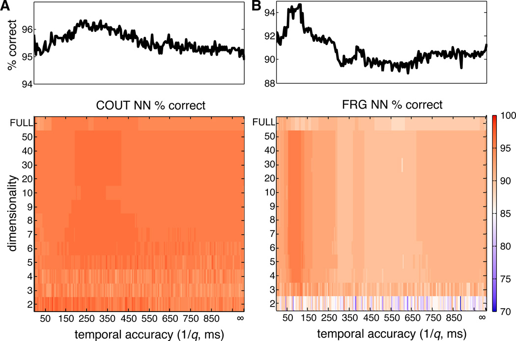
We also examined the effect of SSIMS dimensionality and temporal accuracy (q value) on classification performance. For this part of the analysis, we selected fixed 1-second time windows coinciding with highly informative periods in each task: starting 100 ms before movement onset for COUT and 500 ms before object contact for FRG. While holding spike train duration and temporal offset constant, we examined classification performance as a function of dimensionality and q (Figure 9). For both of the tasks, dimensionality reduction did not have an adverse effect on classification, suggesting that the low dimensional spaces successfully characterize the patterns present in the original high dimensional pair-wise similarity matrix. In the COUT task, 2 dimensions were sufficient for accurate decoding, while in the FRG task performance was more stable with 3 or more dimensions. We explicitly tested clustering without the benefit of dimensionality reduction (labeled as ‘FULL’ dimensionality in Figure 9); for both tasks a modest but consistent increase in classification was observed when dimensionality reduction was applied (more pronounced for the FRG task). Adjusting the temporal resolution of the algorithm (q value) produced different effects in the two tasks examined. Recall that q determines the cost of shifting, such that a shift of more than 1/q has a cost equivalent to removing a spike and inserting a new one. This cutoff determines when the algorithm treats spikes as temporally shifted versions of each other, rather than unrelated events. Changing the value of q had a relatively small effect on classification accuracy for the COUT task. However, there was a gradual trend towards better classification for temporal accuracy values of 250 ms. The FRG task displayed a clearer effect of temporal resolution, with a consistent increase in classification accuracy for 1/q values around 100 ms. Overall, incorporating spike timing provided better performance than assuming a pure rate code (setting q = 0). This finding demonstrated the advantage of incorporating spike timing information rather than only spike counts.

Figure 9. Effect of dimensionality and q on SSIMS.

A. Effect of q and dimensionality on direction classification in the COUT task. In the ‘FULL’ dimensionality condition classification was performed directly on the pairwise distance matrices without applying t-SNE. Infinite temporal resolution corresponds to setting q = 0 (pure rate code). The following parameters were held constant: window start time = −0.1 s, spike train duration = 1 s. The marginal distribution averaging percent correctly classified trials across dimensions is shown above each plot. B. Effect of q and dimensionality on grip classification in the FRG task. Same conventions as A. Window start time = −0.5 s, spike train duration = 1 s.

We also tested the effect of varying the perplexity setting in t-SNE (which determines the effective number of neighbors for each point). Algorithm performance did not vary for perplexity values between 1 and 50 (data not shown).

4 Algorithm validation using synthetic data

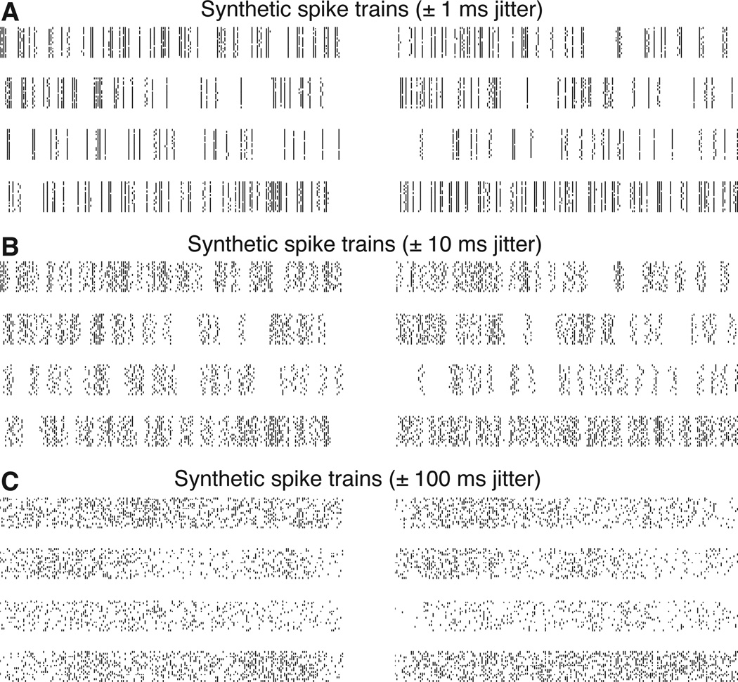
In the two data sets analyzed, classification accuracy showed systematic variation as a function of the q settings in the SSIMS algorithm. However, the true degree of temporal accuracy for the behaviors examined is not known. In order to test whether the SSIMS algorithm is sensitive to the temporal resolution of spiking patterns, we conducted additional tests using synthetic spike trains with predetermined degrees of temporal precision. Artificial data was generated based on eight one-second spike trains recorded from a sample neuron recorded in the COUT data set (one spike train for each movement direction). In order to simulate a stochastic response, synthetic spike trains were generated by applying a random jitter to each recorded spike train (drawn from a uniform distribution) and then removing a percentage of the spikes (chosen randomly between 0 and 20%). The magnitude of the introduced jitter was used as a model for the temporal accuracy of the neural code. Fifty-one synthetic datasets were generated with jitter values ranging from 1 to 500 ms. Each dataset included 20 samples for each of the eight directions. Sample spike trains with varying levels of jitter are shown in (Figure 10).

Figure 10. Synthetic spike trains.

Eight different spike trains recorded in primary motor cortex served as templates for synthetic data generation. For each synthetic dataset each spike train was jittered and randomly subsampled removing between 0 and 20% of the spikes. Samples of spike trains jittered by ±1, 10, and 100 ms are shown in A, B, and C, respectively.

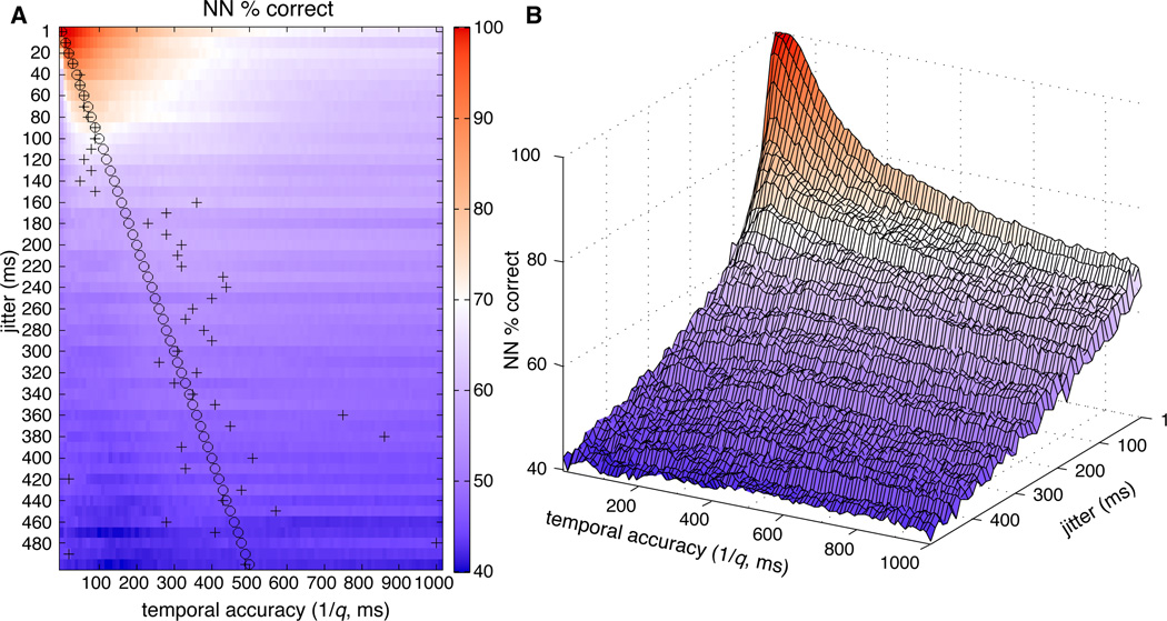
Each synthetic dataset (representing neural codes with varying degrees of temporal consistency) was evaluated in separate runs of the SSIMS algorithm using values of the q parameter ranging from 0 to 1000, resulting in values of 1/q ranging from 1000 (effectively infinite) to 1 ms. For all tests performed, the algorithm yielded above chance classification (with a minimum of 40%, significantly above the expected chance value of 12.5% for eight categories). For jitter values of up to 100 ms, the peak in classification as a function of 1/q closely matched the true temporal accuracy (jitter) of the synthetic data (Figure 11A). This observation shows that the SSIMS algorithm can be used to detect precise temporal patterns in spiking data and estimate their precision. As temporal codes progressively deteriorate (at higher jitter values), classification accuracy becomes less sensitive to the q parameter setting (Figure 11B). These findings suggest that optimization of q is not critical for rate-based codes, but can become an important factor in the discrimination of activity patterns where information is contained in the timing of individual spikes.

Figure 11. Estimating the temporal accuracy of neural codes.

A. Classification accuracy (using a nearest neighbor classifier implemented using leave-one-out cross validation) is plotted as a function of the jitter used to generate the synthetic data (y-axis) and the q value setting for the SSIMS algorithm (x-axis). Classification results shown are the average value obtained across 20 iterations of synthetic data generation. For each synthetic dataset (row) the jitter value is highlighted by a circle. Similarly, the value of 1/q yielding the highest NN classification is highlighted with a ‘+’ sign. B. 3D projection of the data presented in panel A. This view highlights the large effects of q parameter settings on classification of spiking patterns with high temporal accuracy (small jitter). The same variation in q has a much less pronounced effect on low accuracy temporal codes (with hundreds of milliseconds of jitter).

5 Discussion

Although neuronal spiking patterns contain large amounts of information, parameterizing the outputs of individual neurons is challenging, since their activity often reflects complex interactions of multiple (often unknown) variables and noise, leading to trial-by-trial variation that is difficult to characterize. Furthermore, the response properties of individual neurons are not stationary, but instead are subject to rapid context-dependent changes (Donoghue et al., 1990; Sanes et al., 1992; Hepp-Reymond et al., 1999; Moore et al., 1999; Li et al., 2001; Tolias et al., 2005; Stokes et al., 2013). Limiting data analysis to sub-populations of neurons that can be described using relatively simple models may severely distort conclusions drawn from an experiment and disregard important relationships that emerge at large scales. With technological advancements allowing for the simultaneous recording of ensembles approaching thousands of neurons, addressing these challenges is becoming increasingly important (Grewe et al., 2010; Ahrens et al., 2012, 2013). The SSIMS algorithm allows the direct comparison of neuronal firing patterns with minimal assumptions regarding the specific nature of neural encoding of the underlying behavioral task or stimulus presentation. Using a similarity-based methodology circumvents the problems of over and under-parameterization: in effect, the templates used to evaluate spiking activity are supplied by the neuronal data. This relational approach is solely based on the intrinsic properties of neural activity, and does not require a direct mapping between neuronal firing patterns and extrinsic variables (measured in the external world). As highlighted in a recent review by Lehky et al., intrinsic, unlabeled, relational, approaches to neural data analysis provide robust, physiologically plausible encoding models (Lehky et al., 2013). Our results demonstrate the flexibility of intrinsic coding implemented in the SSIMS framework. We were able to apply an almost identical analysis (differing only in the number of categories to discriminate) for neural activity elicited in very different behavioral contexts without having to adjust any parameters relating firing patterns to extrinsic variables. Avoiding the need for ‘extrinsic labeling’ is one of the main features that makes this kind of model appealing from a biological standpoint (Lehky et al., 2013).

Our results also demonstrate how accurate movement decoding (of either reach direction and grip type) can be achieved by applying relatively simple algorithms (such as nearest neighbor classifiers) to SSIMS representations. The algorithm can successfully discriminate between ensemble spiking patterns associated with a planar 8-directional reaching task, accurately reflecting the relationships between reach directions (Figure 3). SSIMS projections can also be used to separate three different grasping strategies used in the Free Reach-to-Grasp task, despite the higher number of degrees of freedom engaged (Figure 5). In both tasks, stable cluster separation was achieved over a broad range of physiologically relevant parameter settings (Figures 8, 9). Classification accuracy was consistently improved by the application of dimensionality reduction as well as the inclusion of spike timing information (Figure 9). This finding highlights the advantages of the two core techniques that form the basis of the SSIMS algorithm. Evaluating neural data under various parameter settings can potentially reveal features related to the inherent dimensionality as well as spike timing precision. In the COUT task, optimal pattern classification was observed with temporal accuracy settings of approximately 250 ms; whereas in the FRG task, classification peaked for 1/q values of approximately 100 ms. Although these observations suggest a greater degree of temporal accuracy for spiking during grasping than reaching behaviors, it must be stressed that the values represent only 2 datasets collected from different animals. Further research involving the comparison of multiple subjects engaged in both tasks would be required to explore this hypothesis. Although pursuing this inquiry is outside the scope of the current manuscript, this finding shows how the application of the SSIMS method can be used to fuel data-driven hypothesis generation. The SSIMS algorithm provides outputs that can be conveniently visualized and quantitatively evaluated. Visual examination of the ensemble SSIMS plots makes it easy to fine-tune algorithm performance: for example, given the overlap between the categories in Figure 3F, we could reasonably expect 100% correct classification for a 4-directional decoder. Of course, this prediction assumes that the properties of the data being recorded are stable over time, an ongoing challenge for on-line neural control (Barrese et al., 2013). SSIMS visualization may also prove useful in this respect, providing and intuitive display of the trial by trial variation of single-unit or ensemble neural activity patterns which would make it easier to detect and address variations in decoder performance. This kind of application may be a valuable tool for the challenge of developing reliable neuromotor prosthetics.

Relationship to existing neural dimensionality reduction algorithms

Evaluating the information content of neuronal ensembles using machine-learning methods for classification and decoding is a widely used strategy. This approach often includes an implicit element of dimensionality reduction: for example, estimating the 2D position of the arm using a Kalman filter (Wu et al., 2006) is a dimensionality reduction operation guided by kinematic parameters. Other algorithms such as population vector decoding (Georgopoulos et al., 1986) can also be viewed as a kinematic-dependent supervised form of dimensionality reduction (since preferred directions must be assigned beforehand). Methods like these require parametrization of neural data with respect to an externally measured covariate. By contrast, relational, intrinsic decoding methods such as SSIMS perform dimensionality reduction in an unsupervised way, with no reference to continuous kinematic variables (Lehky et al., 2013).

Non-supervised dimensionality reduction techniques based on principal component analysis (PCA) have also been successfully used to produce concise representations of neural ensemble activity without a priori knowledge of external variables (Churchland et al., 2007, 2010, 2012; Mante et al., 2013). This approach has revealed structured transitions from movement preparation to execution not evident using traditional analysis methods focusing on single-unit changes in firing rate. Several studies have applied relational encoding methods using multidimensional scaling (MDS) to examine cortical ensemble activity in the primate visual system (Young and Yamane, 1992; Rolls and Tovee, 1995; Op de Beeck et al., 2001; Kayaert et al., 2005; Kiani et al., 2007; Lehky and Sereno, 2007). Murata and colleagues have also employed similar methods to examine grasp-related encoding in area AIP (Murata et al., 2000). These studies have successfully generated low-dimensional spaces representing relational coding of different objects and grip strategies.

One key difference between the SSIMS algorithm and other methods is the combination of dimensionality reduction with spike train similarity metrics. Instead of representing neuronal activity in terms of firing rates (either binned, or smoothed using a kernel function) the SSIMS algorithm applies dimensionality reduction to sets of pair-wise distances between spike trains, allowing for retention of millisecond-level spike timing information. Although it is still necessary to specify a time window, the precise timing of each spike is taken into account; it is therefore possible to examine relatively large time windows without sacrificing temporal resolution. Previous work on spike train metrics revealed no net benefits from the application of dimensionality reduction, aside from convenient visualization (Victor and Purpura, 1997). Our method differs from previous applications in terms of how information from individual neurons is combined. Instead of collapsing ensemble similarity measures by shifting spikes between neurons, our approach keeps information from each neuron segregated until the dimensionality reduction step. Our choice of dimensionality reduction algorithm (t-SNE, as described in van der Maaten and Hinton, 2008) also differs from traditional approaches by using dynamic density estimation to minimize the differences between local neighborhoods in the high and low dimensional spaces.

We directly compared the SSIMS algorithm to methods using MDS or PCA implemented on data represented in terms of spike counts as well as spike train similarity metrics. Our results show an increase in the accuracy of pattern recognition associated with both components of the SSIMS algorithm (Figs. 6 and 7, Table 1). The combination of spike train similarity with t-SNE allow the SSIMS algorithm to effectively use dimensionality reduction to enhance pattern recognition, improving performance compared to the alternative methods tested.

Limitations and future work

The main application for the SSIMS method is the comparison of discrete experimental conditions with the goal of clustering similar activity patterns. SSIMS coordinates are determined by the relative similarity of the activity patterns analyzed. It is therefore not possible to directly map SSIMS projections generated from different ensembles into the same space (for example, from different subjects, or different brain areas). However, normalized clustering statistics (for example the ratio between within and between-cluster distances) could be used to compare SSIMS representations from different ensembles. Decoding results (such as the nearest-neighbor classifier demonstrated here) can also be used to quantify and compare the separation between activity patterns from different sources.

Although the SSIMS method provides useful visualization and quantification of the main trends present in the data, it should not be regarded as a comprehensive representation of all the information contained in a given set of neural activity patterns. For example, time-varying continuous variables may fail to produce clear clusters unless there are underlying repeating motifs centered around the time epochs of interest. Furthermore, while low dimensional representations may reveal the principal organizing patterns for a dataset, more subtle trends may not be evident without taking into account higher dimensional spaces. Note that while this may hinder visualization, the statistical techniques described for cluster evaluation can be used to determine the optimal dimensionality to discriminate patterns in a given task.

For the current implementation of the algorithm, it is necessary to align spike trains using an external reference event, which inevitably introduces temporal jitter related to the sensor and detection system used. Metrics based on inter-spike intervals could help mitigate possible misalignments (Victor and Purpura, 1996). Future versions of the algorithm may also refine spike train alignment using other biological signals, such as local field potentials (for example, in addition to comparing the timing of spikes, it may be useful to compare their phase alignment with respect to ongoing oscillations at specific frequencies). The current metric also lacks an explicit model of potential interactions between different neurons. Incorporating similarity between pairs or neurons, or measures of synchrony between them could potentially expand the sensitivity of the algorithm. Tracking the evolution of SSIMS cluster statistics using sliding time windows, will also be also possible to see how particular activity patterns converge or diverge over time, providing insight into ensemble dynamics.

The t-SNE algorithm is well suited for the separation and classification of neural activity patterns based on pair-wise similarity metrics because of the emphasis it places on comparisons among neighboring points. However, the dynamic density estimation used to define local neighborhoods can potentially have a normalization effect on the variance of individual clusters. Therefore, if the goal of the analysis is to estimate the inherent variability of neural responses in different conditions, it may be better to perform the comparison using other dimensionality reduction methods (or foregoing dimensionality reduction altogether).

Note that to demonstrate the application of SSIMS for classification we used a simple NN method. NN, however, is not a part of the main SSIMS algorithm. Of course, more sophisticated classifiers could be applied to the SSIMS output, likely providing further improvements in decoding accuracy.

Conclusion

Understanding the relationship between patterns of activity emerging in large scale neural recordings is a key step in understanding principles of biological information processing. The SSIMS algorithm provides a widely applicable framework for neural data analysis allowing both straightforward visualization of of an arbitrary number of simultaneously recorded spike trains and a way to perform precise statistical comparisons between activity patterns. By combining spike train metrics that capture precise spike timing and a dimensionality reduction technique based on pair-wise similarity, we have demonstrated that SSIMS is an effective analytical tool in two dramatically different non-human primate experimental paradigms.

The techniques described can be employed beyond the motor domain, providing a way to quantify the relationship between perceptual or cognitive states where kinematics do not provide an intuitive topography. Additionally applying unsupervised clustering algorithms (such as k-means) to SSIMS data could reveal clusters of similar neural activity patterns without any a priori knowledge of the behavioral context. Using these tools, it may be possible to automatically identify recurring network states as well as the transitions between them, providing an intuitive framework to represent the high level flow of neural computation.

References

- Ahrens MB, Li JM, Orger MB, Robson DN, Schier AF, Engert F, Portugues R. Brain-wide neuronal dynamics during motor adaptation in zebrafish. Nature. 2012;485(7399):471–477. doi: 10.1038/nature11057. [DOI] [PMC free article] [PubMed] [Google Scholar]
- Ahrens MB, Orger MB, Robson DN, Li JM, Keller PJ. Whole-brain functional imaging at cellular resolution using light-sheet microscopy. Nat. Methods. 2013;10(5):413–420. doi: 10.1038/nmeth.2434. [DOI] [PubMed] [Google Scholar]
- Alivisatos AP, Chun M, Church GM, Deisseroth K, Donoghue JP, Greenspan RJ, McEuen PL, Roukes ML, Sejnowski TJ, Weiss PS, Yuste R. The brain activity map Science. 2013;339(6125):1284–1285. doi: 10.1126/science.1236939. [DOI] [PMC free article] [PubMed] [Google Scholar]
- Arimura N, Nakayama Y, Yamagata T, Tanji J, Hoshi E. Involvement of the globus pallidus in behavioral goal determination and action specification. J. Neurosci. 2013;33(34):13639–13653. doi: 10.1523/JNEUROSCI.1620-13.2013. [DOI] [PMC free article] [PubMed] [Google Scholar]
- Barrese JC, Rao N, Paroo K, Triebwasser C, Vargas-Irwin C, Franquemont L, Donoghue JP. Failure mode analysis of silicon-based intracortical microelectrode arrays in non-human primates. J. Neural Eng. 2013;10(6):066014. doi: 10.1088/1741-2560/10/6/066014. [DOI] [PMC free article] [PubMed] [Google Scholar]
- Churchland MM, Cunningham JP, Kaufman MT, Foster JD, Nuyujukian P, Ryu SI, Shenoy KV. Neural population dynamics during reaching. Nature. 2012;487(7405):51–56. doi: 10.1038/nature11129. [DOI] [PMC free article] [PubMed] [Google Scholar]
- Churchland MM, Cunningham JP, Kaufman MT, Ryu SI, Shenoy KV. Cortical preparatory activity: representation of movement or first cog in a dynamical machine? Neuron. 2010;68(3):387–400. doi: 10.1016/j.neuron.2010.09.015. [DOI] [PMC free article] [PubMed] [Google Scholar]
- Churchland MM, Yu BM, Sahani M, Shenoy KV. Techniques for extracting single-trial activity patterns from large-scale neural recordings. Curr Opin Neurobiol. 2007;17(5):609–618. doi: 10.1016/j.conb.2007.11.001. [DOI] [PMC free article] [PubMed] [Google Scholar]
- Donoghue JP, Suner S, Sanes JN. Dynamic organization of primary motor cortex output to target muscles in adult rats. ii. rapid reorganization following motor nerve lesions. Exp. Brain Res. 1990;79(3):492–503. doi: 10.1007/BF00229319. [DOI] [PubMed] [Google Scholar]
- Dushanova J, Donoghue J. Neurons in primary motor cortex engaged during action observation. Eur. J. Neurosci. 2010;31(2):386–398. doi: 10.1111/j.1460-9568.2009.07067.x. [DOI] [PMC free article] [PubMed] [Google Scholar]
- Fluet M-C, Baumann MA, Scherberger H. Context-specific grasp movement representation in macaque ventral premotor cortex. J. Neurosci. 2010;30(45):15175–15184. doi: 10.1523/JNEUROSCI.3343-10.2010. [DOI] [PMC free article] [PubMed] [Google Scholar]
- Georgopoulos AP, Kalaska JF, Caminiti R, Massey JT. On the relations between the direction of two-dimensional arm movements and cell discharge in primate motor cortex. J. Neurosci. 1982;2(11):1527–1537. doi: 10.1523/JNEUROSCI.02-11-01527.1982. [DOI] [PMC free article] [PubMed] [Google Scholar]
- Georgopoulos AP, Schwartz AB, Kettner RE. Neuronal population coding of movement direction. Science. 1986;233(4771):1416–1419. doi: 10.1126/science.3749885. [DOI] [PubMed] [Google Scholar]
- Grewe BF, Langer D, Kasper H, Kampa BM, Helmchen F. High-speed in vivo calcium imaging reveals neuronal network activity with near-millisecond precision. Nat. Methods. 2010;7(5):399–405. doi: 10.1038/nmeth.1453. [DOI] [PubMed] [Google Scholar]
- Hepp-Reymond M-C, Kirkpatrick-Tanner M, Gabernet L, Qi HX, Weber B. Context-dependent force coding in motor and premotor cortical areas. Exp. Brain Res. 1999;128(1–2):123–133. doi: 10.1007/s002210050827. [DOI] [PubMed] [Google Scholar]
- Kayaert G, Biederman I, Vogels R. Representation of regular and irregular shapes in macaque inferotemporal cortex. Cereb. Cortex. 2005;15(9):1308–1321. doi: 10.1093/cercor/bhi014. [DOI] [PubMed] [Google Scholar]
- Kiani R, Esteky H, Mirpour K, Tanaka K. Object category structure in response patterns of neuronal population in monkey inferior temporal cortex. J. Neurophysiol. 2007;97(6):4296–4309. doi: 10.1152/jn.00024.2007. [DOI] [PubMed] [Google Scholar]
- Lehky SR, Sereno AB. Comparison of shape encoding in primate dorsal and ventral visual pathways. J. Neurophysiol. 2007;97(1):307–319. doi: 10.1152/jn.00168.2006. [DOI] [PubMed] [Google Scholar]
- Lehky SR, Sereno ME, Sereno AB. Population coding and the labeling problem: extrinsic versus intrinsic representations. Neural Comput. 2013;25(9):2235–2264. doi: 10.1162/NECO_a_00486. [DOI] [PubMed] [Google Scholar]
- Li C-SR, Padoa-Schioppa C, Bizzi E. Neuronal correlates of motor performance and motor learning in the primary motor cortex of monkeys adapting to an external force field. Neuron. 2001;30(2):593–607. doi: 10.1016/s0896-6273(01)00301-4. [DOI] [PubMed] [Google Scholar]
- Li N, DiCarlo JJ. Unsupervised natural visual experience rapidly reshapes size-invariant object representation in inferior temporal cortex. Neuron. 2010;67(6):1062–1075. doi: 10.1016/j.neuron.2010.08.029. [DOI] [PMC free article] [PubMed] [Google Scholar]
- Mante V, Sussillo D, Shenoy KV, Newsome WT. Context-dependent computation by recurrent dynamics in prefrontal cortex. Nature. 2013;503(7474):78–84. doi: 10.1038/nature12742. [DOI] [PMC free article] [PubMed] [Google Scholar]
- Moore CI, Nelson SB, Sur M. Dynamics of neuronal processing in rat somatosensory cortex. Trends. Neurosci. 1999;22(11):513–520. doi: 10.1016/s0166-2236(99)01452-6. [DOI] [PubMed] [Google Scholar]
- Murata A, Gallese V, Luppino G, Kaseda M, Sakata H. Selectivity for the shape, size, and orientation of objects for grasping in neurons of monkey parietal area aip. J. Neurophysiol. 2000;83(5):2580–2601. doi: 10.1152/jn.2000.83.5.2580. [DOI] [PubMed] [Google Scholar]
- Op de Beeck H, Wagemans J, Vogels R. Inferotemporal neurons represent low-dimensional configurations of parameterized shapes. Nat. Neurosci. 2001;4(12):1244–1252. doi: 10.1038/nn767. [DOI] [PubMed] [Google Scholar]
- Pearce TM, Moran DW. Strategy-dependent encoding of planned arm movements in the dorsal premotor cortex. Science. 2012;337(6097):984–988. doi: 10.1126/science.1220642. [DOI] [PMC free article] [PubMed] [Google Scholar]
- Rao NG, Donoghue JP. Cue to action processing in motor cortex populations. J Neurophysiol. 2014;111(2):441–453. doi: 10.1152/jn.00274.2013. [DOI] [PMC free article] [PubMed] [Google Scholar]
- Rigotti M, Barak O, Warden MR, Wang X-J, Daw ND, Miller EK, Fusi S. The importance of mixed selectivity in complex cognitive tasks. Nature. 2013;497(7451):585–590. doi: 10.1038/nature12160. [DOI] [PMC free article] [PubMed] [Google Scholar]
- Rolls ET, Tovee MJ. Sparseness of the neuronal representation of stimuli in the primate temporal visual cortex. J. Neurophysiol. 1995;73(2):713–726. doi: 10.1152/jn.1995.73.2.713. [DOI] [PubMed] [Google Scholar]
- Sanes JN, Donoghue JP. Plasticity and primary motor cortex. Annu. Rev. Neurosci. 2000;23:393–415. doi: 10.1146/annurev.neuro.23.1.393. [DOI] [PubMed] [Google Scholar]
- Sanes JN, Wang J, Donoghue JP. Immediate and delayed changes of rat motor cortical output representation with new forelimb configurations. Cereb. Cortex. 1992;2(2):141–152. doi: 10.1093/cercor/2.2.141. [DOI] [PubMed] [Google Scholar]
- Scott SH. Apparatus for measuring and perturbing shoulder and elbow joint positions and torques during reaching. J. Neurosci. Methods. 1999;89(2):119–127. doi: 10.1016/s0165-0270(99)00053-9. [DOI] [PubMed] [Google Scholar]
- Stokes MG, Kusunoki M, Sigala N, Nili H, Gaffan D, Duncan J. Dynamic coding for cognitive control in prefrontal cortex. Neuron. 2013;78(2):364–375. doi: 10.1016/j.neuron.2013.01.039. [DOI] [PMC free article] [PubMed] [Google Scholar]
- Suner S, Fellows MR, Vargas-Irwin C, Nakata GK, Donoghue JP. Reliability of signals from a chronically implanted, silicon-based electrode array in non-human primate primary motor cortex. IEEE Trans. Neural. Syst. Rehabil. Eng. 2005;13(4):524–541. doi: 10.1109/TNSRE.2005.857687. [DOI] [PubMed] [Google Scholar]
- Tolias AS, Keliris GA, Smirnakis SM, Logothetis NK. Neurons in macaque area v4 acquire directional tuning after adaptation to motion stimuli. Nat. Neurosci. 2005;8(5):591–593. doi: 10.1038/nn1446. [DOI] [PubMed] [Google Scholar]
- van der Maaten LJP, Hinton GE. Visualizing high-dimensional data using t-SNE. Journal of Machine Learning Research. 2008;(9):2579–2605. [Google Scholar]
- Vargas-Irwin C, Donoghue JP. Automated spike sorting using density grid contour clustering and subtractive waveform decomposition. J. Neurosci. Methods. 2007;164(1):1–18. doi: 10.1016/j.jneumeth.2007.03.025. [DOI] [PMC free article] [PubMed] [Google Scholar]
- Vargas-Irwin CE, Shakhnarovich G, Yadollahpour P, Mislow JMK, Black MJ, Donoghue JP. Decoding complete reach and grasp actions from local primary motor cortex populations. J. Neurosci. 2010;30(29):9659–9669. doi: 10.1523/JNEUROSCI.5443-09.2010. [DOI] [PMC free article] [PubMed] [Google Scholar]
- Victor JD. Spike train metrics. Curr Opin Neurobiol. 2005;15(5):585–592. doi: 10.1016/j.conb.2005.08.002. [DOI] [PMC free article] [PubMed] [Google Scholar]
- Victor JD, Purpura KP. Nature and precision of temporal coding in visual cortex: a metric-space analysis. J. Neurophysiol. 1996;76(2):1310–1326. doi: 10.1152/jn.1996.76.2.1310. [DOI] [PubMed] [Google Scholar]
- Victor JD, Purpura KP. Metric-space analysis of spike trains: theory, algorithms and application. Network: Computation in Neural Systems. 1997;8(2):127–164. [Google Scholar]
- Wu W, Gao Y, Bienenstock E, Donoghue JP, Black MJ. Bayesian population decoding of motor cortical activity using a kalman filter. Neural Comput. 2006;18(1):80–118. doi: 10.1162/089976606774841585. [DOI] [PubMed] [Google Scholar]
- Young MP, Yamane S. Sparse population coding of faces in the infer-otemporal cortex. Science. 1992;256(5061):1327–1331. doi: 10.1126/science.1598577. [DOI] [PubMed] [Google Scholar]