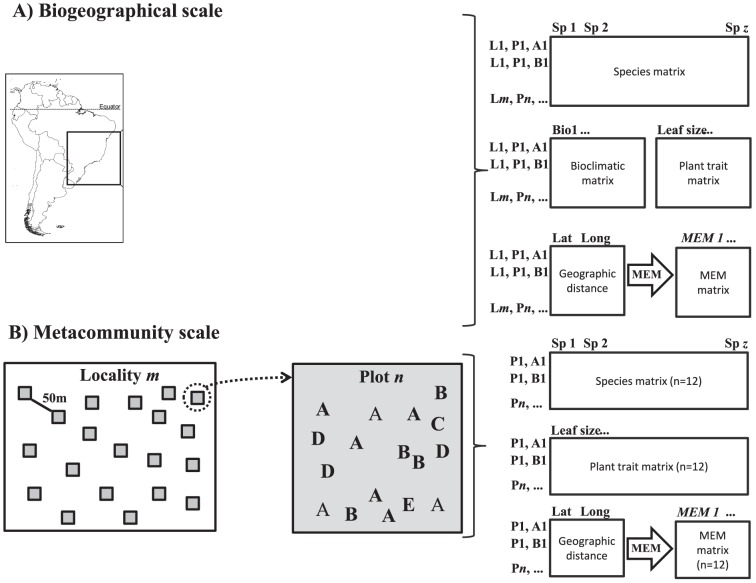
Figure 1. Multiple scales used in the study.

A) Map of South America (left) and the geographical range of the study (middle). The symbols present each 12 sampled localities; localities with similar symbols (grey squares, black triangles and grey circles) have similar climatic characteristics (Fig. S1 in S1 Appendix). From Northeast to South, the order of the sampled localities is the same as in Table 1. Each row of the local matrices (n = 12 per arthropod group) presents the sampled plot (Pn) and individual plant (A, B, C, D or E_{1 to 20}) (1B, right). At the biogeographical scale (1A, middle), we used a species matrix (including all localities), two groups of environmental variables (climate and plant architectural features), and the distance among plots to perform the RDA_{biogeographical} (right); thus, we ran one RDA_{biogeographical} for each arthropod group. Each row of the regional matrix presents the locality (Lm), the plot (Pn), and the individual plant (A, B, C, D or E_{1 to 20}) (1A, right). B) Representation of sampling procedure showing the distribution of twenty plots (30×30 m, grey squares) in the locality m (left), as well as the minimum distance between plots (i.e., 50 m). We sampled up to five individual plants per plant species (A, B, C, D, and E) in each plot. At the metacommunity scale (1B, left), we used a species matrix, only plant architectural features as environmental variables, and the distance among n plots to perform the RDA_{metacommunity}; thus, we ran 12 RDA_{metacommunity} for each arthropod group (see Table 1). See additional details about the definition of biogeographical and metacommunity scales, as well as the analytical procedure in Methods.