Figure 2. High-resolution structures of DEBS domains are consistent with their solution-state structures.

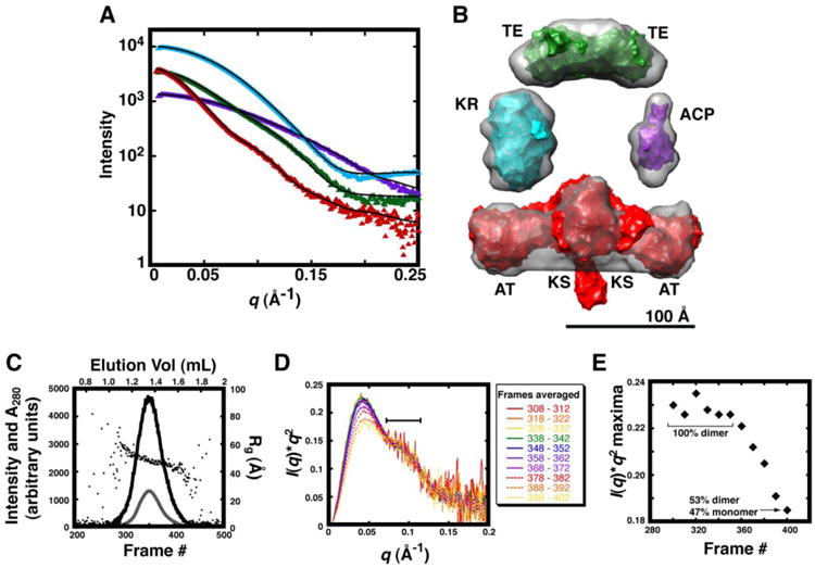
(A). Experimental data collected for holo-ACP3, KR1, TE, and KSAT3 are plotted as purple, cyan, green, and red triangles, respectively. Each atomic resolution structure was treated as a rigid body, and terminal regions such as the polyhistidine tag were modeled with CORAL. For this, the NMR structure of apo-ACP2 is compared with holo-ACP3 and the crystal structures of KR1, the TE domain, and KSAT3 are compared with scattering data collected for KR1, the TE domain, and KSAT3, respectively. Theoretical scattering curves for the resulting models were fit to experimental data in CRYSOL, and the resulting curves are shown as black lines with χ_holo-ACP3 = 6.56, χ_KR1 = 3.35, χ_TE = 5.59, and χ_KSAT3 = 1.91. Chi²-free values were also tabulated as indicated in Table S4. (B) The surface of each atomic-resolution structure is colored as in (A) and fit into the average molecular envelopes (grey) calculated in DAMMIF. (C) SAXS datasets were collected every 5 sec along the SEC elution profile of KSAT3. The A₂₈₀ (grey line) peak and SAXS I(0) (black line) were aligned following data collection, and plotted along with corresponding R_g values (black circles). I(0) and R_g were calculated using Guinier analysis. (D) Every five consecutive scattering curves were averaged, transformed into Kratky plots, and scaled along the q-region highlighted with a bar (70-115 Å^-1). (E) The peak position in each Kratky curve from (D) is plotted according to the frame number of each exposure along the SEC elution profile; the resulting plot shows a partial two-state transition. The fraction of monomeric and dimeric species was estimated using OLIGOMER with the KSAT3 crystal structure modeled to include the N-terminal docking domain. Datasets from the plateau in the left-hand portion of the plot (314-326) were averaged, and used in subsequent analysis. The averaged scattering curve used for structural modeling is shown in Figure S8.