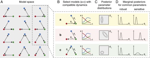
Fig. 1.

Overview of TSA applied to parameter inference. (A) Model space includes our initial candidate model and a series of altered topologies that are consistent with our chosen rules (e.g., all two-edge, three-node networks, where nodes indicate species and directed edges show interactions). One topology may correspond to one or several ODE models depending on the parametric forms we choose to represent interactions. (B) We test each ODE model to see whether it can generate dynamics consistent with our candidate model and the available experimental data. For TSA, we select a group of these compatible models and compare the conclusions we would draw using each of them. (C) Associated with each model m is a parameter space ${\Theta }_m$ (gray); using Bayesian methods we can infer the joint posterior parameter distribution (dashed contours) for a particular model and dataset. (D) In some cases, equivalent parameters will be present in several selected models (e.g., ${\theta }_1$, which is associated with the same interaction in models a–c). We can compare the marginal posterior distribution inferred using each model for a common parameter to test whether our inferences are robust to topological changes, or rely on one specific set of model assumptions (i.e., sensitive). Different models may result in marginal distributions that differ in position and/or shape for equivalent parameters, but we cannot tell from this alone which model better represents reality—this requires model selection approaches (2–4).