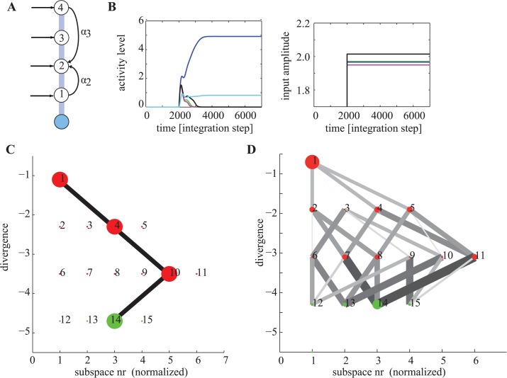
Figure 5. Steering of computation.

(A) The same network as shown in Fig. 4A, with two additional excitatory connections α ₂ = 0.2 and α ₃ = 0.2. (B) Simulation of an individual run. Top shows the state and bottom the inputs to the network. Although the input is identical to Fig. 4B, the computation proceeds differently due to presence of the additional connections. (C) Trajectory through state space for the simulation shown in (C). The state space trajectory is initially identical to the simulation shown in (Fig. 4C), but then diverges. (D) All transitions made by the network. The transition probabilities are now biased and non-equal. Consequently, some permitted subspaces are reached more frequently than others.