Figure 5.

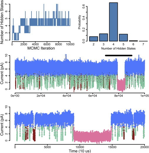
Application of iAMM to BK data. (Top row) Relating to posterior distribution of number of hidden states; it seems that this data has four hidden states. (Middle) Data trace labeled for the hidden states. The iAMM finds one open state (blue), and three closed states. For the closed states, the fastest timescale state (green) is different enough from a slower one (red) that we are able to identify them as distinct. Additionally, an extremely slow closed state (pink) is identified. (Bottom) Same data at an expanded scale. Algorithm parameters: α = 1, γ = 1, and κ = 100.