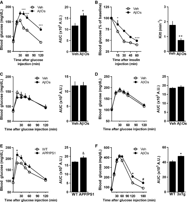
Figure 1.
AD mouse models show peripheral glucose intolerance
- Adult Swiss mice (n = 11 Veh; 15 AβOs) received a single i.c.v. injection of vehicle or 10 pmol AβOs and were assessed in a glucose tolerance test (2 g glucose/kg body weight, i.p.) 7 days after injection. Blood levels of glucose were measured at several time points following glucose administration. Bar graph represents areas under the curves in the time course plot. Data are representative of three independent experiments with similar results. Left panel: ***P = 0.0006, two-way ANOVA followed by Bonferroni post hoc test; right panel: *P = 0.0207, Student's t-test.
- Insulin tolerance test (1 IU insulin/kg body weight, i.p.) (n = 7 Veh; 8 AβOs). Blood levels of glucose were measured at several time points following insulin administration. Bar graph represents the kinetic constants for glucose disappearance (Kitt) calculated from the time course plot. Data are representative of two independent experiments with similar results. Left panel: *P = 0.0456 and ***P = 0.0007, two-way ANOVA followed by Bonferroni post hoc test; right panel: **P = 0.0033, Student's t-test.
- Glucose tolerance test (2 g glucose/kg body weight, i.p.) in mice 7 days after a single intracaudal (C; n = 8 animals/group) or intraperitoneal (D; n = 13 animals/group) injection of AβOs (10 pmol) or vehicle.
- Glucose tolerance test (2 g glucose/kg body weight, i.p.) in 8- to 13-month-old APP/PS1 mice (E; n = 9 animals/group) or 6-month-old 3xTg-AD male mice (F; n = 10 WT; 9 3xTg), or their corresponding wild-type littermates. Bar graph represents areas under the curves in the time course plots. In (E), left panel: *P = 0.0466, two-way ANOVA followed by Bonferroni post hoc test; right panel: &P = 0.072, Student's t-test. In (F), left panel: *P = 0.0171 and #P = 0.0781, two-way ANOVA followed by Bonferroni post hoc test; right panel: *P = 0.0101, Student's t-test.
Data information: Data are expressed as means ± SEM.

