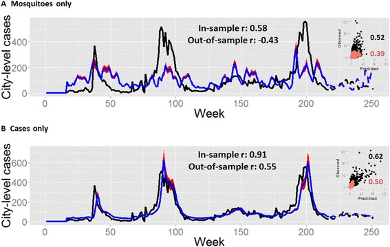
Figure 3.

City-level summary of model fits for Vitoria. The best model with only mosquito covariates, M _i and ∑ _j M _j, (A) is compared to the best model with only dengue-case covariates, Y _i and ∑ _j (Y _j f(x _j )) (B). Models were fitted using neighborhood-level data but aggregated to the city level for presentation. Goodness-of-fit was calculated as the Spearman’s correlation (r) between the observed and model-predicted values for the fitted model (“In-sample”, solid lines) and out-of-sample predictions (dashed lines). Correlation coefficients are presented for both the aggregated city-level data (main plots) and for the neighborhood-level results presented in the scatterplot insets. Observed data (black lines; solid: in-sample, dashed: out-of sample); model predictions (blue lines; solid: in-sample, dashed: out-of sample), 97.5% credible intervals (red shades: in-sample; pink shades: out-of-sample). (A) Y _i,t = β ₁ M _i,t-13 + β ₂∑_j M _j,t-12 ^0.1 + log(P _i) + π _i (B) Y _i,t = β ₁ Y _i,t-1 + β ₂∑_j(Y _j,t-1 /d _ij ) ^0.5 + log(P _i) + π _i; only the best Y _j term is presented (although they are all similar). For both models, the best lag and scale terms were included as indicated (lag terms are a mean from a 3-week window, e.g., 13 represents the mean for weeks 13–15). Y are cases, M are mosquitos, P is population size, π is the neighborhood random effect, t is the week, i is the target neighborhood and j are the sum of all other neighborhoods that are not i.