Analysis of Replication Timing Using Synchronized Budding Yeast Cultures

Abstract

Eukaryotic DNA replication exhibits at once extraordinary fidelity and substantial plasticity. The importance of the apparent presence of a replication temporal program on a population level has been the subject of intense debate of late. Such debate has been, to a great extent, facilitated by methods that permit the description and analysis of replication dynamics in various model organisms, both globally and at a single-molecule level. Each of these methods provides a unique view of the replication process, and also presents challenges and questions in the interpretation of experimental observations. Thus, wider applications of these methods in different genetic backgrounds and in different organisms would doubtless enable us to better understand the execution and regulation of chromosomal DNA synthesis as well as its impact on genome maintenance.

1 Introduction

Eukaryotic chromosomal DNA replication, on a cell-population level, follows a temporal order, i.e., certain regions of the chromosome replicate before others during S phase of the cell cycle [1]. Because such a temporal order is readily observed from yeast to humans [2, 3], it is inferred that a well-executed temporal program of replication is crucial for the fidelity of chromosome maintenance and partition. Indeed, altered replication timing has been linked to increased genome instability in yeast [4–6] and, in metazoans, to transcription [7, 8], cell differentiation [4, 9–12], and cancer formation [13–15]. Thus, it is of great importance to understand how the replication temporal program is executed and regulated. The execution of this replication temporal program involves the coordination of hundreds to thousands of origins of replication in the genome, the sites where replication initiates [16, 17]. Therefore, the replication temporal program is a complex result of the many variables associated with each origin location, efficiency of initiation, and the contentious intrinsic timing of initiation [18–20]. Naturally, in order to understand its function and regulation it is important to observe and describe the replication temporal program in experimental systems.

Genome-wide analyses of replication timing have been described in various eukaryotes from yeast to humans [21]. Here, we focus on a modified approach of the classic Meselson/Stahl density transfer coupled with microarray. This technique is based on the separation of replicated from unreplicated DNA in a density gradient and their subsequent labeling and co-hybridization on a microarray, in order to study replication timing of synchronized budding yeast cells (Fig. 1). Variations of this method have previously been applied in diverse genetic backgrounds to describe a variety of replication timing-associated phenotypes [4, 5, 19, 22–24]. Labeling DNA with dense-isotope-substituted nitrogen and carbon sources is deemed relatively less disruptive than labeling with nucleotide analogs such as BrdU [25], although not as benign as simply measuring the increase in copy number as different segments of the genome are replicated. On the other hand, the density transfer method may offer higher sensitivity and resolution than monitoring DNA copy number changes [26]. Thus, the density transfer method permits global analysis of replication timing in yeast strains of virtually any genetic background, though with greater ease in strains that are: (1) prototrophic for uridine and adenine synthesis, as mutations in these biosynthesis pathways lead to inefficient uptake of the substituted isotopes in genomic DNA, and (2) of the mating type a so as to facilitate cell cycle synchronization via the mating pheromone α-factor.

Fig. 1.

Overview of procedures for density transfer coupled with microarray. Sample graphs for slot-blot, replication kinetics, and Chromosome VI replication profile are all derived from a W303 culture at 25 °C. The dot on the x-axis of the replication profile denotes the centromere. % Rep % replication

2 Materials

2.1 Cell Culture Sample Collection

All solutions are autoclaved or filter sterilized unless otherwise noted.

1. AGD H₂O (autoclaved glass-distilled H₂O). Prepare all solutions in AGD H₂O unless otherwise noted.

2. “-N” Medium: 1.61 g/L YNB (Yeast nitrogen base) without (NH₄)₂SO₄ and without amino acids, 94 mM succinic acid, 167 mM NaOH.

3. Dense Medium: 0.1 % d-Glucose-¹³C₆ (Sigma) and 0.01 % Ammonium-¹⁵N₂ sulfate (Sigma) in “-N” Medium (see ^{Note 1}). Supplement with required amino acids.

4. “Y complete” Medium, pH 5.8: 14.5 g/L YNB without (NH₄)₂SO₄ and without amino acids, 10 g/L succinic acid, 6 g/L NaOH, 5 g/L (NH₄)₂SO₄, 20 g/L glucose, 76.7 mg/L adenine, 76.7 mg/L histidine, 76.7 mg/L methionine, 76.7 mg/L uracil, 76.7 mg/L arginine, 191.8 mg/L phenylalanine, 230.1 mg/L lysine, 230.1 mg/L tyrosine, 306.8 mg/L tryptophan, 306.8 mg/L leucine, 306.8 mg/L isoleucine, 383.6 mg/L glutamic acid, 383.6 mg/L aspartic acid, 575.3 mg/L valine, 767.1 mg/L threonine, 1534.2 mg/L serine (see ^{Note 2}).

5. α-factor (peptide sequence: NH₂–WHWLQLKPGQPMY–COOH, custom synthesized by ThermoFisher at >70 % purity): Prepare as 200 μM or 3 mM stocks (1,000× stocks) for bar1 and BAR1 strains, respectively. Store at −80 °C.

6. Bioruptor Standard Model (Diagenode).

7. 500-mL centrifuge bottles.

8. Centrifuge with JA-10 and JA-17 rotors.

9. Pronase.

10. 10 % NaN₃.

11. 0.2 M EDTA pH 8.0.

12. Frozen (−20 °C) EDTA/NaN₃ Mix: 0.1 % NaN₃, 0.2 M EDTA pH 8.0 (see ^{Note 3}).

13. Nalgene 50-mL Oak Ridge high-speed centrifuge tubes.

14. 500-mL screw-cap centrifuge bottles.

15. Cold 100 % ethanol, stored at −20 °C.

2.2 Flow Cytometry

1. Cold AGD H₂O, stored at 4 °C.

2. 50 mM sodium citrate pH 7.4.

3. 1 mg/mL RNase A, stored at −20 °C.

4. 20 mg/mL proteinase K: 50 % Glycerol, 10 mM Tris–HCl pH 7.5, 19.73 μM CaCl₂, 20 mg/mL Proteinase K, stored at −20 °C.

5. 1 μM SYTOX Green in 50 mM sodium citrate, prepared fresh.

6. Bioruptor Standard Model (Diagenode).

7. BD flow cytometry tubes (Becton Dickinson): 5-mL polystyrene round-bottom tubes for flow cytometric acquisition.

8. BD LSRFortessa flow cytometry analyzer (Becton Dickinson).

9. FlowJo software (Tree Star, Inc.) for data analysis.

10. Microscope slides and cover glasses.

2.3 Genomic DNA Isolation, EcoRI Restriction Digestion, and Southern Hybridization

1. Glass beads, acid washed 425–600 μm (Sigma-Aldrich), autoclaved.

2. 25:24:1 phenol:chloroform:isoamyl alcohol, stored at 4 °C.

3. Lysis buffer: 10 mM Tris–HCl pH 8.0, 1 mM EDTA pH 8.0, 100 mM NaCl, 1 % SDS, 2 % Triton X-100.

4. 100 % ethanol, stored at room temperature.

5. Cold 70 % ethanol, stored at −20 °C.

6. TE_0.1: 10 mM Tris–HCl, 0.1 mM EDTA pH 8.0.

7. 1 mg/mL RNase A, stored at −20 °C.

8. 1 M Tris–HCl, pH 7.5.

9. 5 M NaCl.

10. 100 mM MgCl₂.

11. 1 % Triton X-100.

12. EcoRI.

13. 10× TBE: 850 mM Tris–Base, 890 mM boric acid, 30 mM EDTA pH 8.3.

14. 1× TBE: dilute from 10× TBE.

15. 0.8 % agarose gel: 8 g/L agarose and 0.3 μg/mL ethidium bromide in 1× TBE.

16. Electrophoresis buffer: 1× TBE, 0.3 μg/mL ethidium bromide.

17. Materials for standard Southern analysis.

2.4 CsCl Gradient Preparation by Ultracentrifugation, Fractionation, Slot-Blot Analysis, and Replication Kinetic Data Processing

1. T₁₀E₁₀₀ pH 7.5: 10 mM Tris–HCl, 100 mM EDTA, 75 mM NaOH, filter-sterilized (see ^{Note 4}).

2. CsCl solution: Weigh T₁₀E₁₀₀ pH 7.5 and CsCl powder at a ratio of 1:1.292 and dissolve the CsCl in T₁₀E₁₀₀ (see ^{Note 5}). Prepare fresh.

3. Refractometer (Zeiss or Bausch & Lomb).

4. 13 × 51 mm or 16 × 45 mm Quick-seal tubes (Beckman Z11207SCA or Z00729SCA), (see Subheadings 3.4.1 and 3.4.2).

5. Pasteur pipette.

6. Quick-Seal sealer (Beckman 358312).

7. Beckman VTi 65.2 or Ti 70.1 rotor.

8. Ultracentrifuge.

9. 96-well plates.

10. 1 M NaOH, stored in polypropylene containers at 4 °C.

11. Template Sealing Foil (Fisher Scientific).

12. 20× SCP: 600 mM Na₂HPO₄, 20 mM EDTA pH 8.0, 2 M NaCl pH 6.8.

13. 10× SCP: dilute from 20× SCP with AGD H₂O.

14. Multichannel pipette.

15. Minifold II Slot-Blot system (Schleicher & Schuell).

16. Whatman 3MM blotting paper (Whatman) for the Minifold II Slot-Blot system.

17. Genescreen™ Hybridization Transfer Membrane (Perkin Elmer), cut to the same size as the Whatman paper.

18. UV crosslinker (e.g., UVP HL-2000 HybriLinker™).

19. Radioisotope imaging and quantification system (e.g., Typhoon phosphorimager and storage phosphor screen).

20. IgorPro 6.3 software (WaveMetrics) or equivalent for data deconvolution.

21. Kaleidagraph 4.1 software (Synergy) or equivalent for replication kinetics curve fitting.

2.5 DNA Labeling and Microarray Hybridization

1. Cold 70 % ethanol, stored at −20 °C.

2. TE: 10 mM Tris–HCl, 1 mM EDTA pH 8.0.

3. 2.5× labeling reaction buffer: 125 mM Tris–HCl pH 6.8, 12.5 mM MgCl₂, 25 mM β-mercaptoethanol, 750 μg/mL random hexamers, stored at −20 °C.

4. 10× dNTP mix: 1.2 mM dATP, 1.2 mM dCTP, 1.2 mM dGTP, 0.6 mM dTTP, 10 mM Tris–HCl pH 8.0, stored at −20 °C.

5. 1 mM Cy5- and Cy3-dUTP (GE Healthcare).

6. 50,000 units/mL Klenow Fragment (3′–5′ exo-) (NEB).

7. QIAquick PCR Purifcation Kit (Qiagen).

8. Nanodrop ND-2000 spectrophotometer (Thermo Scientific).

9. Agilent 4 × 44K ChIP to chip yeast microarrays.

10. Feature Extraction software (Agilent).

11. Microarray hybridization and scanning facility.

2.6 Generation of Replication Profiles

1. A file containing a list of genomic coordinates (chromosome number and coordinate) for the microarray probes that will be used in the analysis (e.g., excluding probes corresponding to mitochondrial DNA). For convenience, we shall call this file “ProbeCoordinates.txt”. The list should be sorted by ProbeID (ascending order), one line per probe, and saved preferably as a tab-delimited text file. Sorting by ProbeID should result in the list also being sorted by chromosome number and coordinate. To allow easy computer processing, chromosome numbers should be in Arabic numerals even though the convention for budding yeast is to use Roman numerals for chromosome numbers. This file needs to be prepared only once for each particular microarray platform, and can subsequently be used for all experiments using that platform. Typically, we prepare this list by performing a batch BLAST search of the yeast genome using the vendor-provided list of probe sequences, discarding all sequences that show either more than one match to the genome or less than a perfect match. From the BLAST results, we extract the chromosome number and coordinate for the left end of the probe. The first row of the file should have column headers. The columns for chromosome number, coordinate (kb), and coordinate (bp) should be labeled “Chr”, “Coord_kb”, and “Coord_bp” (without the quotes) to match the file manipulations in Subheading 3.6, step 16.

2. A file containing a list of probes to exclude from the final analysis (e.g., probes corresponding to Ty element sequences), formatted as above. Again, this file needs to be prepared only once for each microarray platform.

3. The statistical software package R, available online at <http://cran.r-project.org/>.

4. The following set of commands saved as a plaintext file to be run in R (see Subheading 3.6, step 16); name the file (for example) “rep_smoothing.R” (see ^{Note 6}):

   # R script for loess smoothing of density transfer data

   files <- list.files(path = “path_to_%replication_files”, full.names =TRUE)

   for(i in seq(along=files)) {

   dataIn <- read.delim(files[i])

   attach(dataIn)

   rep.loess <- loess(Percent_rep ∼ Coord_kb, dataIn, span = winSize/tail(Coord_kb, n=1))

   rep.predict <- predict(rep.loess, Coord_kb)

   dataOut <- data.frame(Chr, Coord_kb, Coord_bp, HLraw, HHraw, Percent_rep, Percent_rep_loess=rep.predict)

   write.table(dataOut, files[i], quote=FALSE, sep= “\t”, eol= “\r”, row.names = FALSE)

   detach(dataIn)

   }

3 Methods

3.1 Sample Collection (Day 1)

1. Grow yeast cells in Dense Medium at 25 °C for at least eight generations. For kinetic measurements with slot-blot analysis only, each sample requires 20 mL of culture; samples for micro-array analysis require >200 mL of culture (see ^{Note 7}).

2. Add a-factor to the log phase culture (at OD₆₆₀ = 0.25) to a final concentration of 200 nM or 3 μM for bar1 or BAR1 strains, respectively.

3. Continue growing the cells until the percentage of unbudded cells reaches >90 % (see ^{Note 8}).

4. Transfer the cells into sterile 500-mL centrifuge bottles and centrifuge in a JA-10 rotor at 1,600 × g for 10 min at 25 °C to collect cell pellets (see ^{Note 9}).

5. Wash the cell pellets with appropriate volumes of “Y-complete” Medium containing 200 nM or 3 μM of a-factor for bar1 or BAR1 strains, respectively, and centrifuge again for 10 min.

6. Resuspend the cell pellets with “Y-complete” Medium with 200 nM or 3 μM of a-factor for bar1 or BAR1 strains, respectively, at a similar volume as that of the cell culture before centrifugation in step 4; continue culturing for another 30 min at 25 °C.

7. Add pronase to the culture at 0.02 mg/mL or 0.3 mg/mL for bar1 or BAR1 strains, respectively, to release cells from a-factor arrest (see ^{Note 10}).

8. Harvest cell samples at a series of time points: pour 20 mL or 200 mL (for slot-blot and microarray analysis, respectively) of the culture into a clean graduated cylinder with 20 μL or 200 μL of 10 % NaN₃ already added, respectively. Quickly mix and transfer the cells onto frozen EDTA/NaN₃ Mix stored in either 50-mL Oak Ridge tubes or 500-mL bottles. Immediately vortex or shake to chill the cells.

9. Store the samples in an ice bath until all samples are collected and follow steps 10–15 for further processing. Remove 1 mL from each sample for flow cytometry and budding index analysis and store in the ice bath until all samples are collected and follow steps 16–18 for further processing.

10. Centrifuge the samples in either a JA-17 (50-mL Oak Ridge tubes) or JA-10 (500-mL bottles) at 1,600 × g for 10 min at 4 °C.

11. Wash the cells with 10 mL of cold AGD H₂O and centrifuge again.

12. Discard the supernatant and transfer the cell pellets with residual liquid into 1.5-mL microcentrifuge tubes or 50-mL tubes, for culture size of 20 or 200 mL, respectively.

13. Centrifuge in a table-top microcentrifuge at 2,500 × g or in a swinging bucket rotor at 2,500 × g for the microcentrifuge tubes or the 50-mL tubes, respectively, for 5 min at 4 °C.

14. Resuspend the cells in 1 or 10 mL of cold AGD H₂O, for culture size of 20 or 200 mL, respectively, and centrifuge again as described in step 13 above.

15. Aspirate the supernatant and store the cell pellets at −20 °C until ready for DNA isolation.

16. For the 1-mL sample collected for FACS and budding index analyses (see step 9 above), centrifuge at 2,500 × g in a micro-centrifuge for 5 min at 4 °C.

17. Wash the cells in 1 mL of cold AGD H₂O and centrifuge again.

18. Add 300 μL of cold AGD H₂O to resuspend the cells, and then add 700 μL of cold 100 % ethanol, while vortexing slowly to mix (see ^{Note 11}). Store the samples at 4 °C.

3.2 Flow Cytometry and Budding Index Analyses

3.2.1 Flow Cytometry Analysis (Day 2–3)

1. Transfer 500 μL from the 1-mL cell sample (see Subheading 3.1, step 18) to a new 1.5-mL microcentrifuge tube and centrifuge at 5,000 rpm for 5 min at 4 °C.

2. Wash the cells in 1 mL of 50 mM sodium citrate pH 7.4 and centrifuge again.

3. Resuspend the cells in 1 mL of 50 mM sodium citrate pH 7.4 containing 50 μg/mL RNase A.

4. Incubate the cells for 1 h at 55 °C.

5. Add 50 μL of 20 mg/mL proteinase K to the cells and continue incubation for 1 h at 55 °C.

6. Centrifuge the cells at 2,500 × g for 5 min at 4 °C.

7. Add 1 mL of the 1 μM SYTOX green solution to resuspend the cells.

8. Incubate the cells in the dark overnight at 4 °C.

9. Sonicate the cells to reduce clumping by a Bioruptor Standard Model on “Low” setting, 30 s on and 30 s off, for two cycles at 4 °C in the dark. Probe sonicator is also acceptable, at a user-defined setting.

10. Transfer the cells to BD flow cytometry tubes and analyze samples on a BD LSRFortessa Flow Cytometry Analyzer, under the Blue Laser (488 nm excitation) with a BP filter at 530 nm emission. The user can also refer to instrument- specific flow cytometry procedures published elsewhere for data acquisition.

11. Analyze the data by FlowJo (Fig. 2) or equivalent.

Fig. 2.

Cell cycle progression of a synchronized W303 culture exiting from α-factor arrest at 25 °C analyzed by flow cytometry. Time after release from the block is indicated. “1C” and “2C” indicate positions of DNA contents in G1 and G2 cells, respectively

3.2.2 Budding Index Analysis (Day 2)

1. Transfer 200 μL from the 1-mL cell sample (see Subheading 3.1, step 18) to a fresh 1.5-mL microcentrifuge tube and centrifuge at 2,500 × g for 5 min at 4 °C.

2. Resuspend the cells in 1 mL of AGD H₂O.

3. To eliminate cell clumping, sonicate them with a Bioruptor Standard Model on “Low” setting, 30 s on and 30 s off, for two cycles at 4 °C. Probe sonicator is also acceptable, at a user-defined setting.

4. Centrifuge the cells at 2,500 × g in a microcentrifuge for 5 min at 4 °C and aspirate most of the water (residual liquid should be less than 20 μL).

5. Resuspend the cells with the residual liquid.

6. Pipette 2 μL of cells and spot on a microscope slide, cover with a cover glass.

7. Count at least 200 cells and note the number of budded cells and unbudded cells.

8. Calculate the budding indices and plot as a function of time (Fig. 3):

   Budding Index = number of budded cells ÷ total number of cells.

9. The maximum budding index could be used to normalize microarray data (see Subheading 3.6).

Fig. 3.

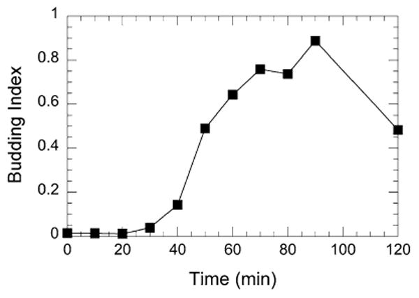
Budding indices of a W303 culture exiting the G1 arrest by α-factor at the indicated times at 25 °C

3.3 Genomic DNA Isolation, EcoRI Restriction Digestion, and Southern Hybridization (Day 4–7)

The following steps are specific for cell pellets collected from 20-mL cell samples. Scale up by fivefold for 200-mL cell culture samples until step 13 below. Perform restriction digestion in the same volume (100 μL) for the 200-mL culture samples as for the 20-mL culture samples.

1. Add 0.3 g of glass beads, 0.2 mL of lysis buffer, and 0.2 mL of 25:24:1 phenol:chloroform:isoamyl alcohol to each frozen cell pellet stored in a 1.5-mL microcentrifuge tube from Subheading 3.1, step 15.

2. Vortex at top speed for 3 min (see ^{Note 12}).

3. Add 0.2 mL of TE and vortex for 10 s at top speed.

4. Centrifuge at >17,000 × g in a microcentrifuge for 5 min at room temperature.

5. Transfer the upper aqueous phase to a fresh 1.5-mL microcentrifuge tube.

6. Add 0.2 mL of lysis buffer to the original tube and repeat steps 2–4.

7. Transfer and combine the upper aqueous phase with that collected in step 5.

8. Add two volumes of room temperature 100 % ethanol and mix thoroughly.

9. Centrifuge at >17,000 × g in a microcentrifuge for 5 min at room temperature and discard the supernatant.

10. If processing the samples (in 50-mL tubes) collected from 200-mL cultures, transfer 1 mL of the mix (see step 8 above) to a 1.5-mL microcentrifuge tube and perform step 9. Transfer another 1 mL of the mix to the same tube and repeat step 9 until the entire mix is processed. This step ensures maximum yield of genomic DNA.

11. Rinse the DNA pellets with 0.5 mL of cold 70 % ethanol by letting the liquid flow onto the pellet side of the tube slowly.

12. Centrifuge at >17,000 × g in a microcentrifuge for 5 s and discard the supernatant.

13. Leave the cap open and air-dry the DNA pellets at room temperature for ∼20 min.

14. Dissolve DNA in 50 μL of TE_0.1 with 50 μg/mL of RNase A and incubate at 37 °C for 30 min. The DNA can be stored at 4 °C; or, continue to EcoRI digestion.

15. For each DNA sample (50 μL), make the EcoRI digestion reaction mix (total 50 μL for each DNA sample) by mixing 10 μL of 1 M Tris–HCl, pH 7.5, 1 μL of 5 M NaCl, 5 μL of 100 mM MgCl₂, 2.5 μL of 1 % Triton X-100, 20 U of EcoRI, and AGD H₂O to the final volume of 50 μL (see ^{Note 13}).

16. Add the 50-μL EcoRI digestion reaction mix to each of the 50-μL DNA samples.

17. Incubate the restriction digestion reaction overnight at 37 °C.

18. Add 1 μL of fresh EcoRI enzyme to the restriction digestion reaction and continue incubation for another 2 h.

19. Transfer the sample to 4 °C to stop the reaction.

20. Analyze 4 μL from the 100-μL restriction digestion reaction on a 0.8 % agarose gel in Electrophoresis buffer (Fig. 4a; see ^{Note 14}).

21. Use standard Southern blot procedures to check the level of digestion with an appropriate DNA probe hybridizing to an average size EcoRI fragment (∼3 kb). If the digestion is incomplete, ethanol precipitate the DNA and repeat the restriction digestion until it reaches >90 % completion (Fig. 4b).

Fig. 4.

Ethidium bromide-stained agarose gel and Southern analysis of EcoRI-digested genomic DNA. (a) Genomic DNA (lanes 2–5) isolated from 200 mL of W303 culture was digested with EcoRI and 0.5 % of the total DNA (0.5 μL from a 100 μL restriction digestion reaction) was separated on a 0.8 % agarose gel. Lane 1, X/Hind III and (Φ×174/HaeIII DNA marker with sizes of DNA fragment in base-pair (bp) as indicated. (b) Southern analysis using the TRP1 gene as a probe

3.4 CsCl Gradient Preparation, CsCl Gradient Fractionation, Slot-Blot Analysis, and Replication Kinetic Data Processing

3.4.1 CsCl Gradient Preparation by Ultracentrifugation Using the Vertical Rotor VTi 65.2 (Day 8–9)

Ultracentrifugation can be done in the vertical rotor VTi 65.2 (described in this section) or the fxed-angle rotor Ti 70.1 (described in Subheading 3.4.2). Comparison of CsCl gradient formation using these rotors is shown in Fig. 5.

Fig. 5.

Comparison of gradient formation of identical DNA samples isolated from a W303 culture at 90 min after release from α-factor arrest, through ultracentrifugation using two different Beckman rotors: the VTi 65.2 rotor (a) and the Ti 70.1 rotor (b). Centrifugation conditions are described in the protocol. Deconvoluted “HH” and “HL” DNA peaks from the slot-blot data are as shown

1. Weigh 9.141 g CsCl solution in a 15-mL tube and mix with 90 μL of EcoRI restriction digestion reaction mix from Subheading 3.3, step 19.

2. Transfer the CsCl and DNA mix into a 13 × 51 mm Quick-seal tube with a Pasteur pipette and use “dummy digestion mix” (EcoRI digestion reaction mix without DNA, mixed with CsCl as described in step 1) to fill up the tube.

3. Seal the tube by a Quick-Seal sealer or a heated flat spatula.

4. Centrifuge at 275,444 × g for 18 h at 20 °C and then at 71,388 × g for 3.5 h at 20 °C, setting the deceleration at transition to “0” (no brakes) and at the end to “1” (transition speed 170 rpm).

3.4.2 CsCl Gradient Preparation by Ultracentrifugation Using the Fixed-Angle Rotor Ti 70.1 (Day 8–9)

1. Weigh 10.97 g CsCl solution in a 15-mL tube and mix with 90 μL of EcoRI restriction digestion reaction mix from Subheading 3.3, step 19.

2. Transfer the CsCl and DNA mix into a 16 × 45 mm Quick-Seal tube with a Pasteur pipette and use “dummy digestion mix” to fill up the tube.

3. Seal the tube by Quick-Seal sealer or a heated flat spatula.

4. Centrifuge the DNA at 207,346 × g for 48 h at 20 °C, setting the deceleration to “1”.

3.4.3 CsCl Gradient Fractionation, Slot-Blot Analysis, and Replication Kinetic Data Processing (Day 10–12)

1. Carefully remove samples from the centrifuge and the rotor.

2. Fractionate each gradient as follows. Secure the centrifuge tube in the fractionation apparatus. Slowly punch a hole at the bottom of the tube and let the gradient steadily drip into the wells of a 96-well plate with seven drops per well (approximately 170 μL/well) (Fig. 6a; see ^{Note 15}).

3. Transfer an appropriate volume of DNA (e.g., 42 μL for DNA from 20-mL cell samples and 2 μL for DNA from 200-mL samples) from each fraction into a new 96-well plate. Add 40 μL of AGD H₂O to the 2 μL DNA, bringing the final volume to 42 μL for the samples from 200-mL cultures.

4. Add 28 μL of 1 N NaOH to each fraction and mix.

5. Seal the 96-well plate with the Template Sealing Foil and incubate for 1 h at 65 °C.

6. Cool the plate to room temperature.

7. Add 70 μL of 20× SCP to each fraction and mix.

8. Pre-wet the Whatman paper and the membrane with 10× SCP and place them into the Minifold, using two layers of Whatman paper underneath the membrane.

9. Using a multichannel pipetter, pipette 140 μL of 10× SCP into each well of the Minifold first, ensuring sound vacuum- assisted flow, before pipetting the 140-μL samples into the wells, followed by 140 μL of 10× SCP to rinse (see ^{Note 16}).

10. Remove the membrane from the Minifold and crosslink DNA to the membrane with 1200 mJ of ultraviolet light in a Crosslinker.

11. Perform standard hybridization of a random-primed ³²P-labeled genomic DNA probe. An example of the blot is shown (Fig. 6b).

12. Perform image acquisition of the radioactively hybridized membrane. Quantify the intensity of each fraction as “total volume” by ImageQuant 5.1 or equivalent software and generate a gradient profile (Fig. 6c).

13. Deconvolute the twin peaks of signals representing the “HH” (unreplicated) and “HL” (replicated) DNA by using the “Multipeak fitting 2” function in IgorPro. Calculate the area under each of the twin peaks and record as “HH” and “HL”, respectively (Fig. 6d).

14. Calculate the percentage of replication (% Replication) at each time point by the following formula: %Replication = 0.5 × “HL” ÷ (“HH” + 0.5 × “HL”) × 100.

15. Plot the % Replication value over the time with KaleidaGraph 4.1 and then fit the data using the “Sigmoidal” function (m1 = 100, m2 = −4, m3 = 30 and m4 = 0.5) to generate the replication kinetic curve (Fig. 7).

16. Calculate T_rep (the time at which half of the maximum percentage of replication is achieved) for the genomic DNA by using a genomic DNA probe.

17. The maximum percentage of replication will be used to normalize microarray data for f, the fraction of the cell population that was cycling—i.e., that actually entered S phase (see Subheading 3.6):

    $$f=\frac{\text{Maximum}\%\text{Replication}}{100}.$$

Fig. 6.

Drip fractionation and slot-blot analyses for quantifying the “HH” and “HL” DNA. Examples of experimental results were obtained from a W303 strain at 50 min after release from α-factor arrest. (a) The gradient is fractionated by collecting seven drops in each well of a 96-well plate in a zig–zag fashion (shown by the arrows for direction of collection). (b) Slot blot image of the middle 24 fractions of the gradient indicated by red arrows in (a), probed with ³²P-dATP-labeled ARS609 DNA. A priori, all 36 fractions might be slot blotted. (c) “Multiple peak fitting” of the intensity plot of slot blot (b) by IgorPro: black squares represent raw data points. (d) Deconvoluted intensity plot in (c): “HH” and “HL” peaks and the values of the integrated area under the peaks are indicated

Fig. 7.

Fitted replication kinetic curve of genomic DNA from a W303 culture at 25 °C

3.5 DNA Labeling, Microarray Hybridization, and Data Extraction (Day 13–14)

1. Pool those fractions containing an estimated 80 % pure “HH” or “HL” DNA, with <20 % contaminations from each other, based on the gradient profile obtained with a genomic DNA probe. This results in a “HH” and a “HL” DNA sample from each original DNA sample collected at a discrete time. Transfer each of these samples, NOT mixing “HH” and “HL” DNA, into a 50-mL Oak Ridge tube (see ^{Note 17}).

2. Add three volumes of cold 70 % ethanol to each DNA sample and mix thoroughly by swirling.

3. Precipitate the DNA for 30 min at −20 °C.

4. Centrifuge at >12,000 × g for 30 min at 4 °C and discard the supernatant.

5. Wash the DNA pellet with 1 mL of cold 70 % ethanol by letting the liquid flow onto the pellet side of the tube slowly.

6. Centrifuge again and discard the supernatant.

7. Invert the tube and air-dry the DNA pellets for up to 16 h (overnight).

8. Add 50 μL of TE to dissolve the DNA and measure the concentration before storing at −20 °C.

9. Transfer 500 ng “HH” DNA and 500 ng “HL” DNA from each sample collected at a discrete time to a new 1.5-mL microcentrifuge tube. Adjust to a final volume of 21 μL with AGD H₂O.

10. Add 20 μL of 2.5× labeling reaction buffer and denature the DNA at 95–100 °C for 5 min.

11. Quick chill the DNA mix on ice and pulse centrifuge to collect condensation.

12. Add 5 μL of 10× dNTP mix, 3 μL of Cy5- or Cy3-dUTP for “HH” or “HL” DNA, respectively, and 1 μL of 50,000 units/mL Klenow Fragment (3′–5′ exo-).

13. Incubate the labeling reaction mix for 2–3 h at 37 °C in the dark.

14. Mix together the “HH” and “HL” samples for each sample collected at a discrete time and use a QIAquick PCR purification kit to clean up the DNA (follow the manufacturer's instructions), eluting with 45 μL of EB buffer.

15. Measure DNA concentration using a NanoDrop ND-2000 spectrophotometer.

16. Hybridize the labeled DNA onto Agilent ChIP to chip yeast microarray slides following manufacturer's instructions.

17. Extract data with the Feature Extraction software and save as a tab-delimited text file.

3.6 Generating a Replication Profile for Each Chromosome in the Yeast Genome

1. Duplicate the data file from Subheading 3.5, step 17. Leave the original file untouched as an archival copy; give the duplicate file a distinctive name and perform all further manipulations on this duplicate.

2. Open the file in Microsoft Excel (or equivalent) and delete the first rows of descriptors, if any, so that the row of column headers (ProbeID, ProbeName, etc.) becomes the first row.

3. Select all the data in the file and sort by ProbeID (ascending sort).

4. Delete the rows corresponding to hybridization control spots (rows 2–331 for Agilent 4 × 44 ChIP arrays).

5. Delete the rows corresponding to mitochondrial DNA probes (the rows at the end of the data table). Important: Perform this step only if you have eliminated mitochondrial DNA probes from the list of probe coordinates in file ProbeCoordinates.txt (see Subheading 2.6, item 1). If you have retained mitochondrial DNA probe information in Subheading 2.6, item 1, you must retain the corresponding rows in the data file from step 4 of this section. At this point, the number of rows of data in this file should correspond exactly to the number of rows of probe coordinates in file ProbeCoordinates.txt.

6. Optional step: delete columns that you will not be using, so as to reduce the file size and speed subsequent manipulations. Typically, we only retain the following columns: ProbeName, gProcessedSignal, rProcessedSignal, gMedianSignal, rMedian-Signal, gBGMedianSignal, and rBGMedianSignal.

7. With the data still sorted by ProbeID, insert the list of genomic locations (chromosome and coordinates, file ProbeCoordinates from Subheading 2.6, item 1) as the left-most columns in the table (i.e., after this step, the chromosome number will be in column 1 and coordinates as kb and bp will be in columns 2 and 3, respectively). Because the data file (see step 6 above) and the list of coordinates (ProbeCoordinates.txt) were both sorted in ascending order by ProbeID, each row of microarray data is now identified by its genomic location. Save the file as tab-delimited text and continue.

8. Identify the “ProcessedSignal” columns corresponding to the HH-DNA and HL-DNA channels. For example, if HH-DNA was labeled with Cy3, the column corresponding to the HH-DNA signal will be the column labeled “gProcessedSignal”. For convenience and for future manipulations, re-label these two columns in the file as “HHraw” and “HLraw”.

9. Obtain the sum of all the HHraw values (“HHsum”). Likewise, get the sum of the HLraw values (“HLsum”).

10. Calculate the normalization parameter γ as defined by the formula:

    $$\mathrm{\gamma }=\left(\frac{\text{HL}}{\text{HH}}\right)÷\left(\frac{\text{HLsum}}{\text{HHsum}}\right)$$

    where HH and HL are the areas under the HH-DNA and HL-DNA peaks obtained for that sample by slot-blot analysis in Subheading 3.4.3, step 13 (Fig. 6d).

11. Create a new column in the worksheet. For each probe location i in the genome, obtain the corrected value %HL_Corr(i); i.e., the value of %HL for that location, corrected for signal differences between the Cy3 and Cy5 channels:

    $${\text{RawRatio}}_i=\frac{{\text{HLraw}}_i}{{\text{HHraw}}_i}.$$

    $${\text{Ratio}}_{\text{Corr}(i)}={\text{RawRatio}}_i\times \gamma .$$

    $$\%{\text{HL}}_{\text{Corr}(i)}=\left(\frac{{\text{Ratio}}_{\text{Corr}(i)}}{1+{\text{Ratio}}_{\text{Corr}(i)}}\right)100.$$

12. Create a new column in the worksheet. Perform the final normalization step to account for f, the fraction of cells in the population that actually entered S phase (see Subheading 3.4.3, step 17). The maximum budding index observed in Subheading 3.2.2, step 9 can be used as a substitute for f if necessary. For each probe location i, calculate %HL_Norm(i), the normalized %HL, and %Replication_Norm(i), the normalized value of % replication:

    $$\%{\text{HL}}_{\text{Norm}(i)}=\left(\frac{\%{\text{HL}}_{\text{Corr}(i)}}{200f+(1-f)\%{\text{HL}}_{\text{Corr}(i)}}\right)200$$
    $$\%{\text{Replication}}_{\text{Norm}(i)}=\left(\frac{\%{\text{HL}}_{\text{Norm}(i)}}{200-\%{\text{HL}}_{\text{Norm}(i)}}\right)100$$

    Label the column with the normalized percent replication values as “Percent_rep” (without the quotes). Save the file.

13. Use the exclusion list (see Subheading 2.6, item 2) to eliminate the rows corresponding to genomic locations you wish to exclude from the final output (see ^{Note 18}).

14. Split the file by chromosome; i.e., create a set of files, each containing the data for just one chromosome but retaining the column headers (Chr, Coord_kb, etc.) from the source file. Create a sub-folder and save each file as tab-delimited text within that folder. For clarity, save each file with a common base name, differing only in a numerical index indicating the chromosome corresponding to that file (e.g., chr01_rep.txt, chr02_rep.txt, etc.; see ^{Note 19}).

15. Using a text editor, open the text file “rep_smoothing.R” created in Subheading 2.6, item 4. In this file, replace “path_to_%replication_files” with the actual path to the folder containing the files saved after splitting the data by chromosome; retain the quotes surrounding the folder path. Replace “winSize” with the desired smoothing window in kb (but “winSize” should be replaced just by the numerical value of the desired window and should not contain the text “kb”). Typically, for density transfer Profiles, we use a smoothing target window of 18 kb. Save the text file (see ^{Note 20}).

16. Smooth the percent replication data for each chromosome by running the following batch command in the unix shell after navigating to the folder/directory containing the file “rep_ smoothing.R” (see ^{Note 21}): R CMD BATCH rep_smoothing.R. The command will invoke the R commands and apply loess smoothing to the data, appending a column of smoothed data values to the file for each chromosome. The column containing the smoothed % replication values will have the label, “Percent_rep_loess”.

17. Using the graphing application of your choice, plot the data for each chromosome (Percent_rep_loess as a function of Coord_ kb or Coord_bp). Set the x-axis dimension to some constant scaling factor (e.g., 1 cm = 100 kb) such that Profiles for all chromosomes are on the same scale. For a sample plot see Fig. 8.

Fig. 8.

Replication profile of chromosome XIII of a W303 culture at 30 min after exiting α-factor arrest at 25 °C. The dots (positioned from high to low) shown above the profile represent OriDB-curated (http://oridb.org) confirmed, likely and dubious origins, respectively

References

- 1.Lucas I, Feng W. The essence of replication timing: determinants and significance. Cell Cycle. 2003;2(6):560–563. [PubMed] [Google Scholar]
- 2.Yaffe E, Farkash-Amar S, Polten A, Yakhini Z, Tanay A, Simon I. Comparative analysis of DNA replication timing reveals conserved large-scale chromosomal architecture. PLoS Genet. 2010;6(7):e1001011. doi: 10.1371/journal.pgen.1001011. [DOI] [PMC free article] [PubMed] [Google Scholar]
- 3.Muller CA, Nieduszynski CA. Conservation of replication timing reveals global and local regulation of replication origin activity. Genome Res. 2012;22(10):1953–1962. doi: 10.1101/gr.139477.112. [DOI] [PMC free article] [PubMed] [Google Scholar]
- 4.McCune HJ, Danielson LS, Alvino GM, Collingwood D, Delrow JJ, Fangman WL, Brewer BJ, Raghuraman MK. The temporal program of chromosome replication: genome-wide replication in clb5{Delta} Saccharomyces cerevisiae. Genetics. 2008;180(4):1833–1847. doi: 10.1534/genetics.108.094359. [DOI] [PMC free article] [PubMed] [Google Scholar]
- 5.Feng W, Bachant J, Collingwood D, Raghuraman MK, Brewer BJ. Centromere replication timing determines different forms of genomic instability in Saccharomyces cerevisiae checkpoint mutants during replication stress. Genetics. 2009;183(4):1249–1260. doi: 10.1534/genetics.109.107508. [DOI] [PMC free article] [PubMed] [Google Scholar]
- 6.Lengronne A, Schwob E. The yeast CDK inhibitor Sic1 prevents genomic instability by promoting replication origin licensing in late G(1) Mol Cell. 2002;9(5):1067–1078. doi: 10.1016/s1097-2765(02)00513-0. [DOI] [PubMed] [Google Scholar]
- 7.Schubeler D, Scalzo D, Kooperberg C, van Steensel B, Delrow J, Groudine M. Genome-wide DNA replication profile for Drosophila melanogaster: a link between transcription and replication timing. Nat Genet. 2002;32(3):438–442. doi: 10.1038/ng1005. [DOI] [PubMed] [Google Scholar]
- 8.Woodfne K, Fiegler H, Beare DM, Collins JE, McCann OT, Young BD, Debernardi S, Mott R, Dunham I, Carter NP. Replication timing of the human genome. Hum Mol Genet. 2004;13(2):191–202. doi: 10.1093/hmg/ddh016. [DOI] [PubMed] [Google Scholar]
- 9.Ryba T, Hiratani I, Sasaki T, Battaglia D, Kulik M, Zhang J, Dalton S, Gilbert DM. Replication timing: a fingerprint for cell identity and pluripotency. PLoS Comput Biol. 2011;7(10):e1002225. doi: 10.1371/journal.pcbi.1002225. [DOI] [PMC free article] [PubMed] [Google Scholar]
- 10.Hiratani I, Ryba T, Itoh M, Yokochi T, Schwaiger M, Chang CW, Lyou Y, Townes TM, Schubeler D, Gilbert DM. Global reorganization of replication domains during embryonic stem cell differentiation. PLoS Biol. 2008;6(10):e245. doi: 10.1371/journal.pbio.0060245. [DOI] [PMC free article] [PubMed] [Google Scholar]
- 11.Hiratani I, Ryba T, Itoh M, Rathjen J, Kulik M, Papp B, Fussner E, Bazett-Jones DP, Plath K, Dalton S, Rathjen PD, Gilbert DM. Genome-wide dynamics of replication timing revealed by in vitro models of mouse embryo-genesis. Genome Res. 2010;20(2):155–169. doi: 10.1101/gr.099796.109. [DOI] [PMC free article] [PubMed] [Google Scholar]
- 12.Shufaro Y, Lacham-Kaplan O, Tzuberi BZ, McLaughlin J, Trounson A, Cedar H, Reubinoff BE. Reprogramming of DNA replication timing. Stem Cells. 2010;28(3):443–449. doi: 10.1002/stem.303. [DOI] [PubMed] [Google Scholar]
- 13.De S, Michor F. DNA replication timing and long-range DNA interactions predict mutational landscapes of cancer genomes. Nat Biotechnol. 2011;29(12):1103–1108. doi: 10.1038/nbt.2030. [DOI] [PMC free article] [PubMed] [Google Scholar]
- 14.Liu L, De S, Michor F. DNA replication timing and higher-order nuclear organization determine single-nucleotide substitution patterns in cancer genomes. Nat Commun. 2013;4:1502. doi: 10.1038/ncomms2502. [DOI] [PMC free article] [PubMed] [Google Scholar]
- 15.Merrick CJ, Jackson D, Diffley JF. Visualization of altered replication dynamics after DNA damage in human cells. J Biol Chem. 2004;279(19):20067–20075. doi: 10.1074/jbc.M400022200. [DOI] [PubMed] [Google Scholar]
- 16.Masai H, Matsumoto S, You Z, Yoshizawa-Sugata N, Oda M. Eukaryotic chromosome DNA replication: where, when, and how? Annu Rev Biochem. 2010;79:89–130. doi: 10.1146/annurev.biochem.052308.103205. [DOI] [PubMed] [Google Scholar]
- 17.Mechali M. Eukaryotic DNA replication origins: many choices for appropriate answers. Nat Rev Mol Cell Biol. 2010;11(10):728–738. doi: 10.1038/nrm2976. [DOI] [PubMed] [Google Scholar]
- 18.Friedman KL, Brewer BJ, Fangman WL. Replication profile of Saccharomyces cerevisiae chromosome VI. Genes Cells. 1997;2(11):667–678. doi: 10.1046/j.1365-2443.1997.1520350.x. [DOI] [PubMed] [Google Scholar]
- 19.Raghuraman MK, Winzeler EA, Collingwood D, Hunt S, Wodicka L, Conway A, Lockhart DJ, Davis RW, Brewer BJ, Fangman WL. Replication dynamics of the yeast genome. Science. 2001;294(5540):115–121. doi: 10.1126/science.294.5540.115. [DOI] [PubMed] [Google Scholar]
- 20.de Moura AP, Retkute R, Hawkins M, Nieduszynski CA. Mathematical modelling of whole chromosome replication. Nucleic Acids Res. 2010;38(17):5623–5633. doi: 10.1093/nar/gkq343. [DOI] [PMC free article] [PubMed] [Google Scholar]
- 21.Gilbert DM. Evaluating genome-scale approaches to eukaryotic DNA replication. Nat Rev Genet. 2010;11(10):673–684. doi: 10.1038/nrg2830. [DOI] [PMC free article] [PubMed] [Google Scholar]
- 22.Alvino GM, Collingwood D, Murphy JM, Delrow J, Brewer BJ, Raghuraman MK. Replication in hydroxyurea: it's a matter of time. Mol Cell Biol. 2007;27(18):6396–6406. doi: 10.1128/MCB.00719-07. [DOI] [PMC free article] [PubMed] [Google Scholar]
- 23.Vincent JA, Kwong TJ, Tsukiyama T. ATP-dependent chromatin remodeling shapes the DNA replication landscape. Nat Struct Mol Biol. 2008;15(5):477–484. doi: 10.1038/nsmb.1419. [DOI] [PMC free article] [PubMed] [Google Scholar]
- 24.Lian HY, Robertson ED, Hiraga S, Alvino GM, Collingwood D, McCune HJ, Sridhar A, Brewer BJ, Raghuraman MK, Donaldson AD. The effect of Ku on telomere replication time is mediated by telomere length but is independent of histone tail acetylation. Mol Biol Cell. 2011;22(10):1753–1765. doi: 10.1091/mbc.E10-06-0549. [DOI] [PMC free article] [PubMed] [Google Scholar]
- 25.Knott SR, Viggiani CJ, Tavare S, Aparicio OM. Genome-wide replication Profiles indicate an expansive role for Rpd3L in regulating replication initiation timing or efficiency, and reveal genomic loci of Rpd3 function in Saccharomyces cerevisiae. Genes Dev. 2009;23(9):1077–1090. doi: 10.1101/gad.1784309. [DOI] [PMC free article] [PubMed] [Google Scholar]
- 26.Yabuki N, Terashima H, Kitada K. Mapping of early firing origins on a replication profile of budding yeast. Genes Cells. 2002;7(8):781–789. doi: 10.1046/j.1365-2443.2002.00559.x. [DOI] [PubMed] [Google Scholar]