Figure 3.

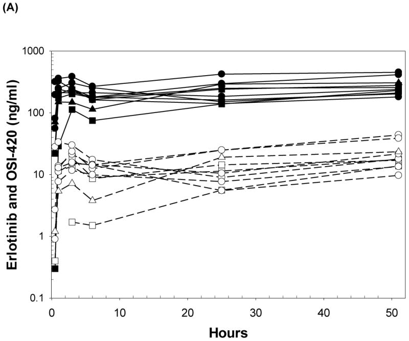
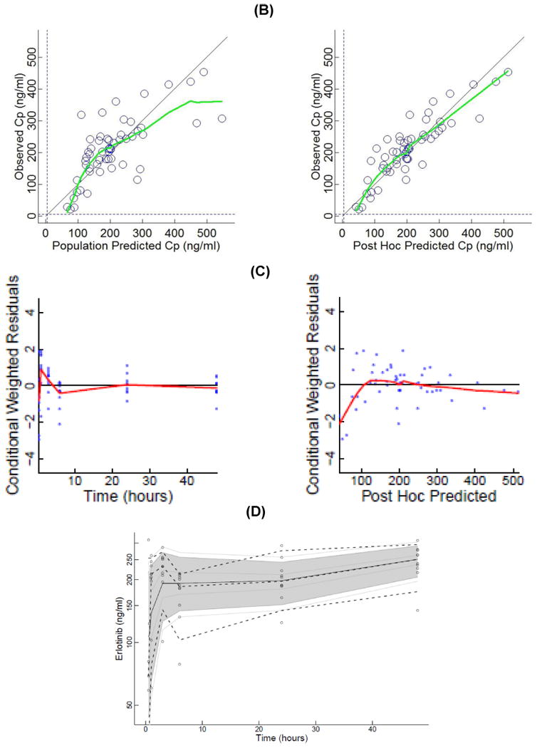
(A) Plasma concentrations of erlotinib and OSI-420 (demethyl erlotinib) versus time. Subjects self-administered 50mg (□, n = 3), 75mg (◯, n = 6) or 100mg erlotinib (Δ, n =1) QD. Closed symbols and solid lines represent erlotinib concentrations, open symbols and dashed lines represent the OSI-420 metabolite. Plasma concentrations of erlotinib were used for PK modeling. (B) Observed versus final model predicted plasma concentrations of erlotinib. The left panel is based on the “typical” prediction without including model variability (IIV), while the right panel is based on the complete model including IIV (post hoc fit). The linear regression coefficients (r², observed versus predicted) for the respective plots were 0.508 and 0.783, respectively. Inclusion of the error model (post hoc model) decreased the standard errors of prediction of the model from 22 to 15%. (C) Conditioned weighted residuals (CWRES) (39) were plotted versus time and post hoc predicted concentrations. The curvilinear plots depict local regression trend smoother fits to the data. The curvilinear plots in C and D depict local regression trend smoother (R Supersmoother) fits to the data. (D) Model validation by “precision corrected visual predictive check” (40), in which observations are normalized to the median (75mg QD) dosing scheme. One thousand simulations were performed per subject and used to compute percentile ranges (P₅, P₂₅, P₅₀, P₇₅ and P₉₅) normalized to median dose and body-weight. Actual observations were also normalized, and superimposed over these ranges for comparison. The shaded area indicates 90% confidence interval; solid lines indicate percentiles: 2.5, 97.5 (red); 5, 95 (blue); 25, 75 (green); 50 (black). Dashed lines indicate percentiles 5, 50, and 95 of observations.