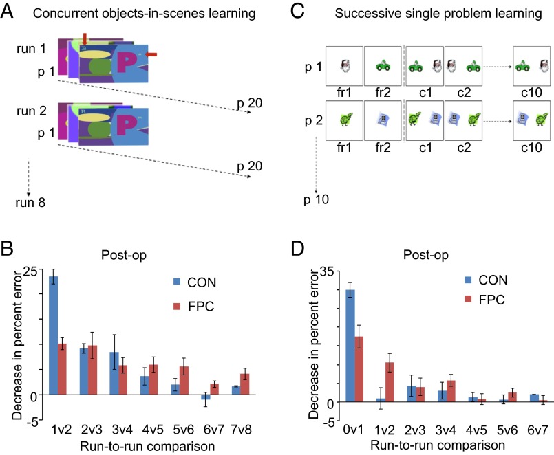
Fig. 2.

Concurrent objects-in-scenes learning and successive single problem learning. (A) Schematic of concurrent objects-in-scenes learning task depicting the relationship between the 20 problems per run (p1 to p20) and the eight runs that make up a daily session (run 1 to run 8). The superimposed red arrows in the figure, not present in the stimuli, indicate the objects’ locations in this example scene. The locations of S⁺ and S⁻ objects in the scene in each problem were fixed. (B) Mean postoperative (Post-op) data plotted separately for the FPC and CON groups, in terms of the run-to-run change in performance [positive values on the y axis indicate improvement between runs (e.g., 1v2 depicts the percentage of erroneous responses on the second run subtracted from the percentage of erroneous responses on the first run)]. (C) Schematic of successive single problem learning task depicting the relationship between the two initial forced response (fr1 and fr2) phases and the 10 subsequent successive choices to this problem (c1 to c10) within each problem, and with 10 problems (p1 to p10) constituting a single session. (D) Postoperative performance for the FPC and CON groups plotted in the same way as in B, depicting improvement across successive attempts at the same problem for the successive single problem learning task (curtailed at 6v7 for comparison with B). All error bars depict ±SEM.