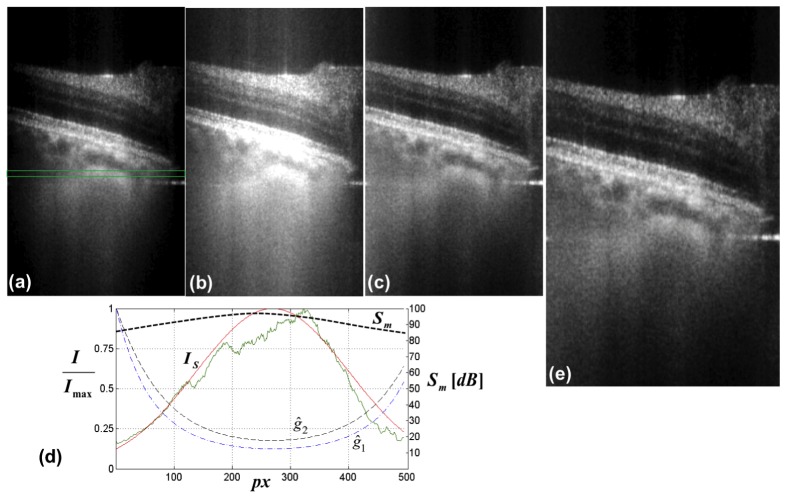
Fig. 7.

Demonstration of the effect of Gaussian weighting on the lateral signal degradation. (a) original retinal tomogram acquired at the periphery of the ONH. The image brightness (B) and contrast (C) was adjusted for optimal examination at the tomogram center. (b) the same tomogram, but B&C adjusted to visualize structures at the periphery. (c) tomogram after lateral Gaussian weighting with curve ${\hat{g}}_1$. (d) normalized lateral signal decay (green curve) as a function of sensor pixels, obtained by averaging over 100 successive sagittal tomograms within the indicated green box in (a). The red curve is the respective Gaussian fit (Sect. 2.3). The normalized black and blue dashed curves ${\hat{g}}_1$ and ${\hat{g}}_2$ are obtained after inverting the Gaussian fit according to Eq. (6) with d = 0 and d = 5 respectively. $S_m$ is the measured lateral sensitivity decay across the sensor pixels. (e) tomogram after Gaussian weighting with curve ${\hat{g}}_2$.