(
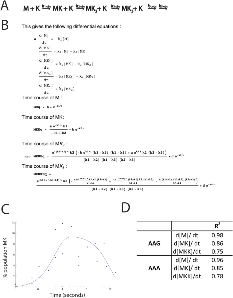
A) Kinetic scheme used to model the rate constants of sequential lysine additions to the peptide chain (same as
Figure 2A). We also attempted to model with peptidyl-tRNA drop-off rates included. Inserting peptidyl-tRNA drop-off into our model decreases the quality of fits, and returns rates of drop-off small enough that they are inconsequential relative to the time scale of the reaction. (
B) The top panel displays the differential equations used to solve for each rate constant. The bottom panels display the mathematical solutions for the differential equations. These solutions were used to perform modeling and fit the data. The fits were performed both iteratively (e.g., we solved for
k1 by fitting the plots measuring the disappearance of M, then input that value into the equation describing the appearance of MK to solve for
k2) and by letting all of the values float for each data set. In both cases, the rate constants modeled were essentially the same, indicating that the first lysine is added quickly (
k1), and subsequent lysines (
k2,
k3) are added more slowly. (
C) An example fit in Mathematica showing time course for the formation and depletion of MK on a message with AAG codons. This time course, for example, was used to model the
k2 value. (
D) R
2 values for the fits for the appearance and disappearance of each species used to model rate constants.


