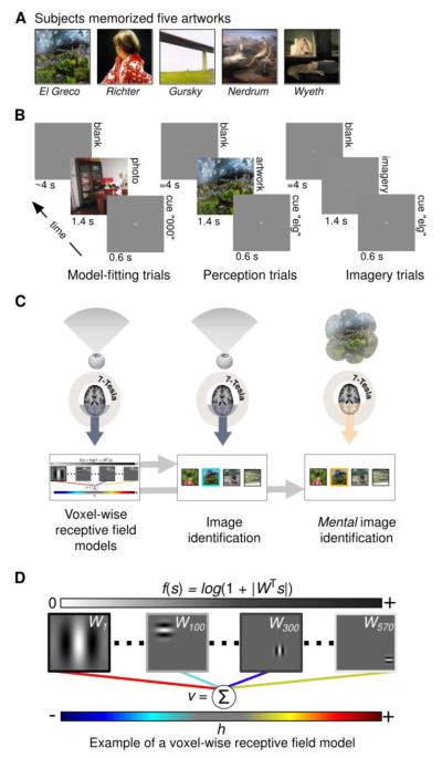
Figure 1. Experimental design.

A) Prior to scanning subjects familiarized themselves with five works of art. B) Scans were organized into separate runs of contiguous trials. During each trial of the model-fitting (left) and model-testing (not shown) runs subjects fixated a central dot while viewing randomly selected photographs (duration of presentation = 1.4 s). Each photograph was preceded by a brief dummy cue (“000”; duration = 0.6 s) and followed by a blank gray screen (mean duration = 4 s). During each trial of the perception runs (middle) subjects viewed only the five works of art. Each artwork was preceded by a distinct 3-letter cue (an abbreviation of the artist’s name) and followed by a blank gray screen (duration = 4 s). Imagery runs (right) were identical to perception runs except that subjects imagined the five works of art while fixating at the center of a gray screen that was 1.4% brighter than the cue screen. C) High-field (7-Tesla) fMRI measurements of BOLD activity in the occipital lobe were obtained during each run. Activity measured during the model-fitting runs (left) was used to construct voxel-wise encoding models (bottom left). The voxel-wise encoding models and activity from the perception runs (middle) were used to perform image identification (bottom middle). The same voxel-wise encoding models and activity from the imagery runs (right) were used to perform mental image identification (bottom right). During image identification a target image (outlined in blue/orange for the perception/imagery runs) is picked out from among a set of randomly selected images. D) A simplified illustration of the voxel-wise encoding model. To produce predicted activity an observed or imagined scene (s) is filtered through a bank of 570 complex Gabor wavelets (represented by the matrix W). Each wavelet is specified by a particular spatial frequency, spatial location, and orientation (four examples shown here). The filter outputs (∣W^Ts∣, where ∣ ∣ denotes an absolute value operation that removes phase information) are passed through a compressive nonlinearity (f(s) = log(1+∣W^Ts∣); outputs are represented by the grayscale bar at top) and then multiplied by a set of model parameters (colored lines; dark to light blue lines indicate negative parameters; yellow to red lines indicate positive parameters). The sum of the weighted filter outputs is the voxel’s predicted activity (v) in response to the stimulus. The model parameters (h) are learned from the training data only and characterize each voxel’s tuning to spatial frequency, spatial location, and orientation.