Figure 5.

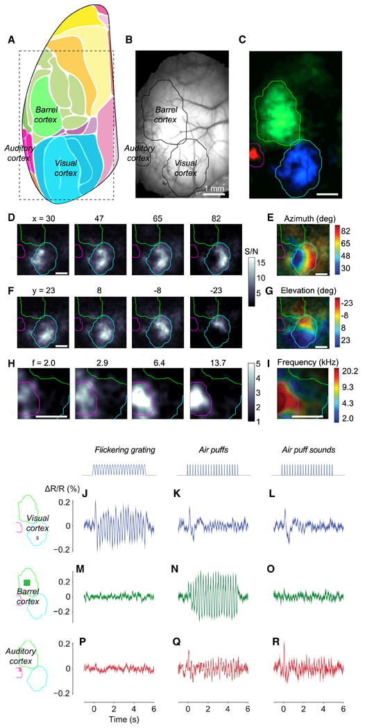
Wide-field imaging of sensory cortices of Ai78 mice expressing VSFP-Butterfly 1.2 in cortical layer 2/3 excitatory neurons. (A) Diagram showing mouse cortical regions observed at an angle of 30° laterally with a vertical optical axis. Adopted and modified from (Kirkcaldie, 2012). The rectangle shows the approximate extent of our imaging area. (B) Fluorescence of mCitrine imaged through the thinned skull. (C) Maps of VSFP signals (acceptor-donor ratio) to auditory (red), somatosensory (green), and visual (blue) stimuli. Sensory regions are mapped as 4 Hz amplitude in response to 4 Hz train of tones, 4 Hz train of air puffs directed to whole whisker field, and 2 Hz flickering visual stimulus. Response amplitude was divided for each modality by amplitude measured in the absence of stimulation. The three maps came from experiments performed on different days, and the resulting maps were aligned based on the blood vessel pattern. Overlaid contour lines show the outlines of visual cortex, barrel cortex, and auditory cortex. (D) Amplitude maps for 4 Hz responses to bars reversing in contrast at 2 Hz, presented at different horizontal positions (azimuths). (E) The resulting maps of azimuth preference (retinotopy). (F-G) Same as D and E for stimulus elevation (vertical position). (H) Amplitude maps for 6 Hz responses to tones in 6 Hz trains, for different tone frequencies. (I) The resulting maps of tone frequency preference (tonotopy). (J-R) Unisensory and multisensory signals in visual cortex (J-L), barrel cortex (M-O) and auditory cortex (P-R). Stimuli were contrast-reversing visual gratings (J, M, P), air puffs delivered to the whiskers (K, N, Q), and (sham) air puffs delivered away from the whiskers to replicate the sound but not the somatosensory stimulation (L, O, R). ΔR/R is calculated after normalization using data during the prestimulus period, and high-pass filtering above 0.5 Hz. (See also Figure S8.)