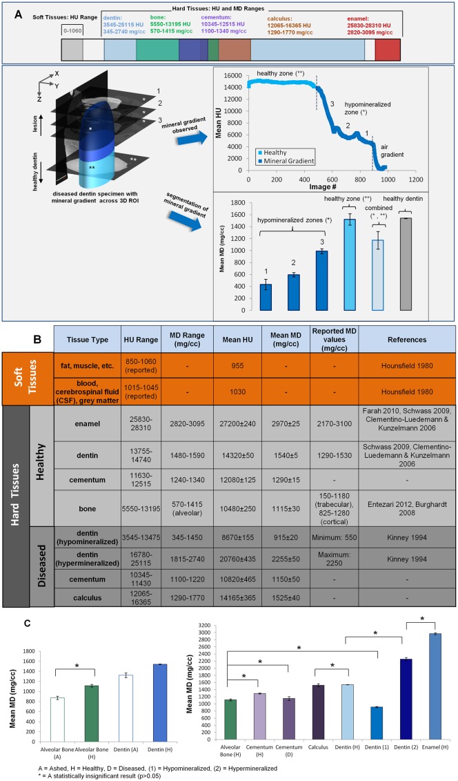
Fig 2. Average HU and MD ranges from experiments and literature.

A) UPPER PANEL: Mineral density and HU ranges of hard and soft tissues and regions of overlap amongst tissues are shown. LOWER PANEL: A schematic of segmentation procedure for diseased tissues, where the upper portion of the 3D volume (dark blue, *) represents lesion volume and the lower portion (medium to light blue, **) is a gradient between lesion shifting to a normal healthy tissue. Mineral gradients through the volume of material are identified by computing mineral density from each 2D virtual slice (e.g. 1, 2, and 3 following procedures highlighted in Fig 1B and 1C). Statistically distinct (p<0.05) hypomineralized zones(*) are decoupled from the observed mineral gradient (upper line plot) for the entire diseased region using segmentation (following procedure highlighted in Fig 1D). The bar chart distinguishes each segmented hypomineralized zone against the healthy zone (**), the combined value (average of both healthy and hypomineralized zones) and healthy dentin; B) Summary of mineral density and HU ranges with average values across hard and soft tissues, including healthy and diseased conditions; C) LEFT PANEL: Mineral density of healthy alveolar bone and dentin calculated by gravimetric and micro-CT. RIGHT PANEL: Calculated mineral density of healthy and diseased hard tissues using a micro-computed tomography unit. To attain mineral density from the data, an ROI through samples was taken for healthy tissues (similar to figs B and C), segmentation was applied for diseased tissues (fig D). Segmented data was compared with ashed mineral density. A = ashed, H = Healthy, D = Diseased, (1) = Hypomineralized, (2) = Hypermineralized, * = A statistically insignificant result (p>0.05), while all other groups not indicated with an asterisk are statistically different.