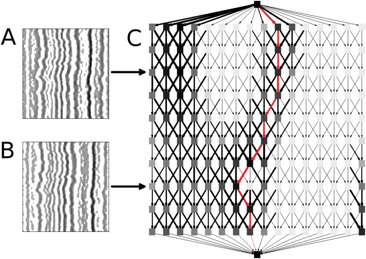
Fig 4. Network assembly.
The Laplacian response image, K, (see Fig 2c) has been rescaled into (A) K D and (B) K B, images that emphasize dark and bright regions in K, respectively. White pixels represent barriers that potential features cannot cross, while continuous dark regions indicate likely features. (C) Here we show one example network, although separate networks are indeed assembled for K B and K D. Each node (square) within the rectangular region represents a pixel in KB or K D. The top and bottom nodes (which we term “peripheral nodes”) are added to provide starting/ending points for the shortest path finding algorithm. The width of the edges corresponds to the inverse of the edge weight, and the darkness of the nodes represents the average weight of incoming edges. The red line illustrates the shortest path through the network. For the sake of visual clarity, this network was created using a small subsection of an actual Laplacian response with k = 1.

