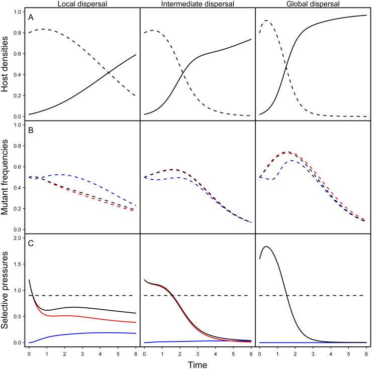
Fig 2. Effect of spatial structure on epidemiology and evolution in the model.
The top figures (A) show simulation results for the density of susceptible (dashed line) and infected hosts (full line) for different level of mixing (left: no mixing (g H = g P = 0), middle: intermediate (g H = g P = 0.5), right: full mixing (g H = g P = 1)). The figures in the middle (B) show simulation results for the change in mutant frequency in the total pathogen population (black), in the horizontally infected hosts (red) or in vertically infected hosts (blue) for different levels of mixing. The figures at the bottom (C) indicate the values of the different components of the selection coefficient identified in Eq (1): the horizontal transmission term (red), the vertical transmission component (blue) and the sum of the previous two terms (black) and the magnitude of the cost of virulence (dashed black). Note that the global mutant frequency increases only when the sum of the transmission terms (full black line) is higher than the cost of virulence (dashed line). Our simulations are the result of the numerical integration of the deterministic approximation of the full spatial model, using Improved Pair Approximation (IPA; [31]) with parameters ϕ = 1/6 and θ = 2/5, which correspond to a triangular lattice (each site has 6 neighbours, see [31] for details). Parameters: α w = 0.1, α m = 1, β w = 2, β m = 3.5, δ = 0.99, d = 0.01. Initial conditions: S(0) = 0.8, ,.

