Unified Heat Kernel Regression for Diffusion, Kernel Smoothing and Wavelets on Manifolds and Its Application to Mandible Growth Modeling in CT Images

Abstract

We present a novel kernel regression framework for smoothing scalar surface data using the Laplace-Beltrami eigenfunctions. Starting with the heat kernel constructed from the eigenfunctions, we formulate a new bivariate kernel regression framework as a weighted eigenfunction expansion with the heat kernel as the weights. The new kernel regression is mathematically equivalent to isotropic heat diffusion, kernel smoothing and recently popular diffusion wavelets. Unlike many previous partial differential equation based approaches involving diffusion, our approach represents the solution of diffusion analytically, reducing numerical inaccuracy and slow convergence. The numerical implementation is validated on a unit sphere using spherical harmonics. As an illustration, we have applied the method in characterizing the localized growth pattern of mandible surfaces obtained in CT images from subjects between ages 0 and 20 years by regressing the length of displacement vectors with respect to the template surface.

1. Introduction

In medical imaging, anatomical surfaces extracted from MRI and CT are often represented as triangular meshes. The image segmentation and surface extraction processes themselves are likely to introduce noise to the mesh coordinates. It is therefore imperative to reduce the mesh noise while preserving the geometric details of the anatomical structures for various applications.

Diffusion equations have been widely used in image processing as a form of noise reduction starting with Perona and Malik since 1990 (Perona and Malik, 1990). Numerous techniques have been developed for surface fairing and mesh regularization (Sochen et al., 1998; Malladi and Ravve, 2002; Tang et al., 1999; Taubin, 2000) and surface data smoothing (Andrade et al., 2001; Chung et al., 2001; Cachia et al., 2003a,b; Chung et al., 2005; Joshi et al., 2009). Isotropic heat diffusion on surfaces has been introduced in brain imaging for subsequent statistical analysis involving the random field theory that assumes an isotropic covariance function as a noise model (Andrade et al., 2001; Chung and Taylor, 2004; Cachia et al., 2003a,b). Since then, isotropic diffusion has been the standard smoothing technique. Such diffusion approaches use finite element or finite difference schemes that are known to suffer numerical instability if a sufficiently small step size is not chosen in the forward Euler scheme.

Iterated kernel smoothing has been another widely used method in approximately solving diffusion equations on surfaces (Chung et al., 2005; Han et al., 2006). Iterated kernel smoothing is often used in smoothing anatomical surface data including cortical curvatures (Luders et al., 2006b; Gaser et al., 2006), cortical thickness (Luders et al., 2006a; Bernal-Rusiel et al., 2008), hippocampus surface (Shen et al., 2006; Zhu et al., 2007) and magnetoencephalography (MEG) (Han et al., 2007) and functional-MRI (Hagler Jr. et al., 2006; Jo et al., 2007) on the brain surface. Due to its simplicity, it is probably the most widely used form of surface data smoothing in brain imaging. In iterated kernel smoothing, kernel weights are spatially adapted to follow the shape of the heat kernel in a discrete fashion along a manifold. In the tangent space of the manifold, the heat kernel can be approximated linearly using the Gaussian kernel for small bandwidth. A kernel with large bandwidth is then constructed by iteratively applying the kernel with small bandwidth. However, this process compounds the linearization error at each iteration.

We propose a new kernel regression framework that constructs the heat kernel analytically using the eigenfunctions of the Laplace-Beltrami (LB) operator, avoiding the need for the linear approximation used by Chung et al. (2005) and Han et al. (2006). The proposed method represents isotropic heat diffusion analytically as a series expansion so it avoids the numerical convergence issue associated with solving the diffusion equations numerically (Andrade et al., 2001; Chung and Taylor, 2004; Joshi et al., 2009). Our framework is different from other existing diffusion-based smoothing methods in that it bypasses the various numerical problems such as numerical instability, slow convergence, and accumulated linearization error.

Although a few studies have introduced heat kernel in computer vision and machine learning (Belkin et al., 2006), they mainly use heat kernel to compute shape descriptors (Sun et al., 2009; Bronstein and Kokkinos, 2010); or to define a multi-scale metric (de Goes et al., 2008). These studies did not use heat kernel in regressing functional data on manifolds. This is the first study that uses heat kernel in the form of regression for the subsequent statistical analysis. There have been significant developments in kernel methods in the machine learning community (Schölkopf and Smola, 2002; Nilsson et al., 2007; Shawe-Taylor and Cristianini, 2004; Steinke and Hein, 2008; Yger and Rakotomamonjy, 2011). However, to our knowledge, heat kernel has never been used in such frameworks. Most kernel methods in machine learning deal with the linear combination of kernels as a solution to penalized regressions. On the other hand, our kernel regression framework does not have a penalized cost function.

Recently, wavelets have been popularized for surface and graph data. For example, spherical wavelets were used on brain surface data that have been mapped onto a sphere (Nain et al., 2007; Bernal-Rusiel et al., 2008). Since wavelet basis has local supports in both space and scale, the wavelet coefficients from the scale-space decomposition using the spherical wavelets provides shape features that describe local shape variation at a variety of scales and spatial locations. However, spherical wavelets require a smooth mapping from the surface to a unit sphere introducing a serious metric distortion, which usually compounds subsequent statistical parametric maps (SPM). Furthermore, such basis functions are only orthonormal for data defined on the sphere and result in a less parsimonious representation for data defined on other surfaces compared to the intrinsic LB-eigenfunction expansion (Seo and Chung, 2011). To remedy the limitations of spherical wavelets, the diffusion wavelet transform on graph data structures has been proposed (Antoine et al., 2010; Coifman and Maggioni, 2006; Hammond et al., 2011; Kim et al., 2012).

The primary methodical contribution of this study is the establishment of a unified regression framework that combines the diffusion-, kernel- and wavelet-based methods for scalar data defined on manifolds. Although diffusion-, kernel- and wavelet-based methods seem to be different methodologies, in this paper we establish a unified framework that relates them in a coherent mathematical fashion by providing detailed theoretical justification. This paper extends the work described in Kim et al. (2011), which introduced heat kernel smoothing to smooth out surface noise in the hippocampus and amygdala. Although the idea of diffusion wavelet transform for surface mesh was explored in Kim et al. (2012), the relationship between the wavelet transform and the proposed kernel regression was not investigated. For the first time, the mathematical equivalence between the two constructs is explained.

The proposed kernel regression framework is subsequently applied in characterizing the growth pattern of the mandible surfaces obtained in CT and identifying the regions of the mandible that show the most significant localized growth. The length of the displacement vector field is regressed over the mandible surface to increase the signal to noise ratio and hence statistical sensitivity. To our knowledge, this is the first growth modeling of the mandible surface in a continuous fashion without using anatomic landmarks.

2. Methods

2.1. Isotropic Diffusion on Manifolds

Consider a functional measurement Y (p) observed at each point p on a compact manifold $\mathcal{M}\subset {\mathbb{R}}^3$. We assume the following linear model on Y :

$$Y\left(p\right)=\theta \left(p\right)+∊\left(p\right).$$ (1)

where θ(p) is the unknown mean signal to be estimated and ε(p) is a zero-mean Gaussian random field. We may assume further $Y\in L^2\left(\mathcal{M}\right)$, the space of square integrable functions on $\mathcal{M}$ with the inner product:

$$\langle f,g\rangle ={\int }_{\mathcal{M}}f\left(p\right)g\left(p\right)d\mu \left(p\right),$$ (2)

where μ is the Lebesgue measure such that $\mu \left(\mathcal{M}\right)$ is the total area of $\mathcal{M}$.

Functional data such as electroencephalography (EEG), magnetoencephalog raphy (MEG) (Han et al., 2007) and functional-MRI (Hagler Jr. et al., 2006; Jo et al., 2007), and anatomical data such as cortical curvatures (Luders et al., 2006b; Gaser et al., 2006), cortical thickness (Luders et al., 2006a; Bernal-Rusiel et al., 2008) and surface coordinates (Chung et al., 2005) can be considered as possible functional measurements. Functional measurements are expected to be noisy and require filtering to boost signal.

Surface measurements have often been filtered using the isotropic diffusion equation of the form (Andrade et al., 2001; Chung et al., 2001; Cachia et al., 2003a; Rosenberg, 1997)

$$\frac{\partial f}{\partial \sigma }=\Delta f,f(p,\sigma =0)=Y\left(p\right),$$ (3)

where Δ is the Laplace-Beltrami operator defined on manifold $\mathcal{M}$. The diffusion time σ controls the amount of smoothing. It can be shown that the unique solution of (3) is given by kernel convolution. This can be easily seen as follows.

A Green's function or a fundamental solution of the Cauchy problem (3) is given by the solution of the following equation:

$$\frac{\partial f}{\partial \sigma }=\Delta f,f(p,\sigma =0)=\delta \left(p\right),$$ (4)

where δ is the Dirac delta function. The heat kernel K_σ is a Green's function of (4) (Evans, 1998), i.e.

$$\frac{\partial K_{\sigma }}{\partial \sigma }=\Delta K_{\sigma },K_{\sigma }(p,\sigma =0)=\delta \left(p\right),$$

Since the differential operators are linear in (4), we can further convolve the terms with the initial data Y such that

$$\frac{\partial }{\partial \sigma }(K_{\sigma }\ast Y)=\Delta (K_{\sigma }\ast Y),K_{\sigma }\ast Y(p,\sigma =0)=Y\left(p\right),$$

where

$$K_{\sigma }\ast Y\left(p\right)={\int }_{\mathcal{M}}{K}_{\sigma }(p,q)Y\left(q\right)d\mu \left(q\right),$$

Hence K_σ * Y is a solution of (3).

2.2. Diffusion Smoothing

Isotropic diffusion (3) has been numerically solved by various numerical techniques (Chung, 2001; Andrade et al., 2001; Cachia et al., 2003a,b; Chung and Taylor, 2004). For diffusion smoothing, the diffusion equation needs to be discretized using the cotan formulation (Chung, 2001; Chung and Taylor, 2004; Qiu et al., 2006). Since there are many different cotan formulations, we followed the formulation first given in Chung (2001). Diffusion equation (3) is discretized as

$$\frac{\partial \mathbf{f}}{\partial \sigma }=-{\mathbf{A}}^{-1}\mathbf{Cf},$$ (5)

where f = (f(p₁, σ), . . . , f(p_n, σ))′ is the vector of measurements over all mesh vertices at time σ. A = (A_ij) is the sti ness matrix and C = (C_ij) is the global coefficient matrix, which is the assemblage of individual element coefficients. The sparse matrices A and C are explicitly given as follows.

Let $T_{ij}^{-}$ and $T_{ij}^{+}$ denote two triangles sharing the vertex p_i and its neighboring vertex p_j in a mesh. Let two angles opposite to the edge containing p_i and p_j be ϕ_ij and θ_ij respectively for $T_{ij}^{+}$ and $T_{ij}^{-}$. The o -diagonal entries of the sti ness matrix are

$$A_{ij}=\frac{1}{12}(\mid T_{ij}^{+}\mid +\mid T_{ij}^{-}\mid )$$

if p_i and p_j and A_ij otherwise. |·| denotes the area of triangle. The diagonal entries are summed as $A_{ii}={\sum }_{j=1}^n{A}_{ij}$. The off-diagonal entries of the global coefficient matrix are

$$C_{ij}=-\frac{1}{2}(\cot {\theta }_{ij}+\cot {\varphi }_{ij})$$

if p_i and p_j are adjacent and C_ij = 0 otherwise. The diagonal entries are similarly given as the sum $C_{ii}=-{\sum }_{j=1}^n{C}_{ij}$

Ordinary differential equation (5) is then further discretized at each point using the forward finite difference scheme:

$$\mathbf{f}(p_i,{\sigma }_{n+1})=\mathbf{f}(p_i,{\sigma }_n)+({\sigma }_{n+1}-{\sigma }_n)\widehat{\Delta }f(p_i,{\sigma }_n),$$ (6)

where $\widehat{\Delta }f(p_i,{\sigma }_n)$ is the estimated Laplacian obtained from the i-th row of −A⁻¹Cf. For the forward Euler scheme to converge, we need to have sufficiently small step size σ = σ_n+1 − σ_n (Chung, 2001).

2.3. Iterated Kernel Smoothing

The diffusion equation (3) can be approximately solved by iteratively performing Gaussian kernel smoothing (Chung et al., 2005). In iterated kernel smoothing, the weights of the kernel are spatially adapted to follow the shape of heat kernel in discrete fashion along a surface mesh. Heat kernel smoothing with large bandwidth can be broken into iterated smoothing with smaller bandwidths (Chung et al., 2005):

$$K_{m\sigma }\ast Y=\underset{m\text{times}}{\underbrace{K_{\sigma }\ast \cdots \ast K_{\sigma }}}\ast Y.$$ (7)

Then using the parametrix expansion (Rosenberg, 1997; Wang, 1997), we approximate the heat kernel with small bandwidth locally using the Gaussian kernel:

$$K_{\sigma }(p,q)=\frac{1}{\sqrt{4\pi \sigma }}\exp [-\frac{d^2(p,q)}{4\sigma }][1+O\left({\sigma }^2\right)],$$ (8)

where d(p, q) is the geodesic distance between p and q. For sufficiently small bandwidth σ, all the kernel weights are concentrated near the center, so the first neighbors of a given mesh vertex are sufficient for approximation. Unfortunately, this approximation is bound to compound error at each additional iteration. For numerical implementation, we used the normalized truncated kernel given by

$$W_{\sigma }(p,q_i)=\frac{\exp [-\frac{d^2(p,q_i)}{4\sigma }]}{{\sum }_{j=0}^r\exp [-\frac{d^2(p,q_j)}{4\sigma }]},$$ (9)

where q₁, . . . , q_r are r neighboring vertices of p = q₀. Denote the truncated kernel convolution as

$$W_{\sigma }\ast Y\left(p\right)=\sum _{i=0}^r{W}_{\sigma }(p,q_i)Y\left(q_i\right).$$ (10)

Then, the iterated heat kernel smoothing is defined as

$$W_{m\sigma }\ast Y\left(p\right)=\underset{m\text{times}}{\underbrace{W_{\sigma }\ast \cdots \ast W_{\sigma }}}\ast Y\left(p\right).$$

2.4. Heat Kernel Regression

We present a new regression framework for solving the isotropic diffusion equation (3). Let Δ be the Laplace-Beltrami operator on $\mathcal{M}$. Solving the eigenvalue equation

$$\Delta {\psi }_j=-\lambda {\psi }_j,$$ (11)

we order eigenvalues

$$0={\lambda }_0<{\lambda }_1<{\lambda }_2<\cdots ,$$

and corresponding eigenfunctions ψ₀, ψ₁, ψ₂, . . . (Rosenberg, 1997; Chung et al., 2005; Lévy, 2006; Shi et al., 2009). Then, the eigenfunctions ψ_j form an orthonormal basis in $L^2\left(\mathcal{M}\right)$. There is extensive literature on the use of eigenvalues and eigenfunctions of the Laplace-Beltrami operator in medical imaging and computer vision (Lévy, 2006; Qiu et al., 2006; Reuter et al., 2009; Reuter, 2010; Zhang et al., 2007, 2010). The eigenvalues have been used in caudate shape discriminators (Niethammer et al., 2007). Qiu et al. used eigenfunctions in constructing splines on cortical surfaces (Qiu et al., 2006). Reuter used the topological features of eigenfunctions (Reuter, 2010). Shi et al. used the Reeb graph of the second eigenfunction in shape characterization and landmark detection in cortical and subcortical structures (Shi et al., 2008, 2009). Lai et al. used the critical points of the second eigenfunction as anatomical landmarks for colon surfaces (Lai et al., 2010). Since the direct application of eigenvalues and eigenfunctions as features of interest is the beyond the scope of the paper, we will not pursue the issue in detail here.

Using the eigenfunctions, heat kernel K_σ(p, q) is defined as

$$K_{\sigma }(p,q)=\sum _{j=0}^{\infty }{e}^{-{\lambda }_j\sigma }{\psi }_j\left(p\right){\psi }_j\left(q\right),$$ (12)

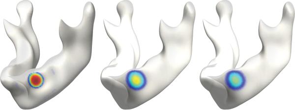
where σ is the bandwidth of the kernel. Figure 1 shows examples of a heat kernel with different bandwidths. Then the heat kernel regression or smoothing of functional measurement Y is defined as

$$K_{\sigma }\ast Y\left(p\right)=\sum _{j=0}^{\infty }{e}^{-{\lambda }_j\sigma }{\beta }_j{\psi }_j\left(p\right),$$ (13)

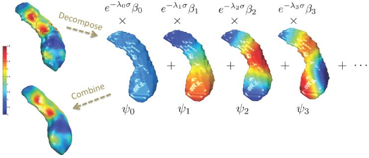
where β_j = 〈Y, ψ_j〉 are Fourier coefficients (Chung et al., 2005) (Figure 2). Kernel smoothing K_σ * Y is taken as the estimate for the unknown mean signal θ. The degree for truncating the series expansion can be automatically determined using the forward model selection procedure.

Figure 1.

Heat kernel shape with bandwidths 0.025 (left), 1.25 (middle) and 5 (right) on a mandible surface. The level sets of the heat kernel form geodesic circles.

Figure 2.

Schematic of heat kernel smoothing. Given functional data on a surface, we compute the eigenfunctions ψ_j and the Fourier coefficients β_j. Then we combine all the terms and reconstruct the functional signal back.

Unlike previous approaches to heat diffusion (Andrade et al., 2001; Chung and Taylor, 2004; Joshi et al., 2009; Tasdizen et al., 2006), our proposed method avoids the direct numerical discretization of the diffusion equation. Instead we discretize the basis functions of the given manifold $\mathcal{M}$ by solving for the eigensystem (11) and obtain λ_j and ψj.

2.5. Diffusion Wavelet Transform

We can establish the relationship between kernel regression and recently popular diffusion wavelets. In fact, it can be shown that the proposed kernel regression is equivalent to the wavelet transform. This mathematical equivalence eliminates the need for constructing wavelets using a complicated computational machinery as has often been done in previous studies (Antoine et al., 2010; Hammond et al., 2011; Kim et al., 2012) and offers a simpler but more unified alternative.

Consider a wavelet basis W_σ,q(p) obtained from a mother wavelet W with scale and translation parameters σ and q respectively in a Euclidean space:

$$W_{\sigma ,q}\left(p\right)=\frac{1}{\sigma }W\left(\frac{p-q)}{\sigma }\right).$$

Generalizing the idea of scaling a mother wavelet in Euclidean space to a curved surface is trivial. However, the difficulty arises when one tries to translate a mother wavelet on a curved surface since it is unclear how to define translation along the surface. If one tries to modify the existing spherical wavelet framework to an arbitrary surface (Nain et al., 2007; Bernal-Rusiel et al., 2008), one immediately encounters the problem of establishing regular grids on an arbitrary surface. Recent works based on the diffusion wavelets bypass this problem by taking the bivariate kernel as a mother wavelet (Antoine et al., 2010; Hammond et al., 2011; Mahadevan and Maggioni, 2006; Kim et al., 2012).

For some scale function g that satisfies the admissibility conditions, diffusion wavelet W_σ,q(p) at position p and scale σ is given by

$$W_{\sigma ,q}\left(p\right)=\sum _{j=0}^{k}q\left({\lambda }_j\sigma \right){\psi }_j\left(p\right){\psi }_j\left(q\right),$$

where λ_j and ϕ_j are eigenvalues and eigenfunctions of the Laplace-Beltrami operator. The wavelet transform is then given by

$$\langle W_{\sigma ,q},Y\rangle ={\int }_{\mathcal{M}}{W}_{\sigma ,q}\left(p\right)Y\left(p\right)d\mu \left(p\right),$$ (14)

If we let g(λ_jσ) = exp(− λ_jσ), we have the heat kernel as the wavelet,

$$W_{\sigma ,p}\left(q\right)=H_{\sigma }(p,q),$$

The bandwidth σ of the heat kernel is the scale parameter, while the translation is done by shifting one argument in the bivariate heat kernel. Subsequently, wavelet transform (14) can then be rewritten as

$$\langle W_{\sigma ,p},Y\rangle =\sum _{j=0}^k{e}^{-{\lambda }_j\sigma }{\beta }_j{\psi }_j\left(q\right)$$ (15)

with β_j = 〈Y, ψ_j〉. The expression (15) is exactly the finite truncation of heat kernel regression in (12). Hence, diffusion wavelet analysis can be simply performed within the proposed heat kernel regression framework without any additional wavelet machinery. We will therefore not distinguish between the heat kernel regression and the diffusion wavelet transform.

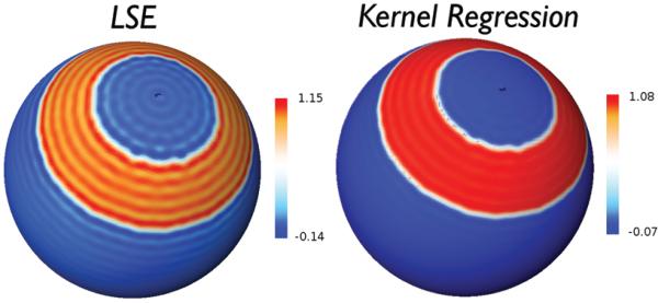
Although the heat kernel regression is constructed using global basis functions ψ_j, surprisingly the kernel regression at each point p coincides with the wavelet transform at that point. Hence, it also inherits all the localization property of wavelets at that point. This is clearly demonstrated in a simulation given in Figure 3, where a step function of value 1 in the circular band 1/8 < θ < 1/4 (angle from the north pole) and of value 0 outside of the band is constructed. Note that on a sphere, the Laplace-Beltrami operator is the spherical Laplacian and its eigenfunctions are spherical harmonics Y_lm of degree l and order m. Then the step function is reconstructed using the spherical harmonic series expansion

$$Y\left(p\right)=\sum _{l=0}^{78}\sum _{m=-l}^l{\beta }_{lm}{Y}_{lm}\left(p\right),$$

where the spherical harmonic coefficients β_lm = 〈Y, Y_lm〉 are obtained by the least squares estimation (LSE). On the unit sphere, we used the heat kernel regression of the form

$$Y\left(p\right)=\sum _{l=0}^{78}\sum _{m=-l}^l{e}^{-l(l+1)\sigma }{\beta }_{lm}{Y}_{lm}\left(p\right)$$

with the small bandwidth σ = 0.0001. The spherical harmonic expansion clearly shows severe ringing artifacts compared to the kernel regression, which inherits the localization power of wavelets. This is why the Gibbs phenomenon is not visibly significant.

Figure 3.

Gibbs phenomenon (ringing artifacts) is visible in the spherical harmonic series expansion with degree 78 via the least squares estimation (LSE) of the step function defined on a sphere. In contrast, the heat kernel regression with the same degree and bandwidth 0.0001 shows less visible artifacts.

2.6. Parameter Estimation in Heat Kernel Smoothing

Since the closed form expression for the eigenfunctions of the Laplace-Beltrami operator on an arbitrary surface is unknown, the eigenfunctions are numerically computed by discretizing the Laplace-Beltrami operator. To solve the eigensystem (11), we need to discretize it on mandible triangular meshes using the cotan formulation (Chung, 2001; Chung and Taylor, 2004; Shi et al., 2009; Qiu et al., 2006; Lévy, 2006; Reuter et al., 2006, 2009; Rustamov, 2007; Zhang et al., 2007; Vallet and Lévy, 2008; Wardetzky, 2008).

Among many different cotan formulations used in computer vision and medical image analysis, we used the formulation given in Chung (2001) and Qiu et al. (2006). It requires discretizing (11) as the following generalized eigenvalue problem:

$$\mathbf{C}\psi =\lambda \mathbf{A}\psi ,$$ (16)

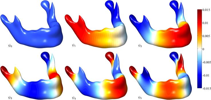
where the global coefficient matrix C is the assemblage of individual element coeffcients and $\mathcal{A}$ are the stiffness matrix. We solved (16) using the Implicitly Restarted Arnoldi Method (Hernandez et al., 2006; Lehoucq et al., 1998) without consuming large amount of memory and time for sparse entries. Figure 4 shows the first few eigenfunctions for a mandible surface. The first eigenfunction is trivially given as λ₀ = 0 and ${\psi }_0=1∕\sqrt{\mu \left(\mathcal{M}\right)}$ for a closed compact surface. It is possible to have multiple eigenfunctions corresponding to a single eigenvalue.

Figure 4.

Eigenfunctions of various degrees for a sample mandible surface. The eigenfunctions are projected on the surface smoothed by the proposed heat kernel smoothing with bandwidth σ = 0.5 and degree k = 132. The smoothed surface is obtained by heat kernel smoothing applied to the coordinates of the surface mesh with the same parameter while preserving the topology of mesh. The first eigenfunction is simply ${\psi }_0=1∕\sqrt{\mu \left(\mathcal{M}\right)}$. The color scale is thresholded for better visualization.

Once we obtain the eigenfunctions numerically, we estimate the kernel regression parameters β_j by minimizing the sum of squared residual using the least squares estimation (LSE):

$$\arg \underset{{\beta }_0,\cdots ,{\beta }_k}{\min }{\Vert Y\left(p\right)-\sum _{j=0}^k{e}^{-{\lambda }_j\sigma }{\beta }_j{\psi }_j\left(p\right)\Vert }^2.$$ (17)

The least squares method is often used in estimating the coefficients in spherical harmonic expansion (Shen et al., 2004; Styner et al., 2006; Chung et al., 2008). Suppose we have n mesh vertices p₁, . . . , p_n. Let

$$\mathbf{Y}={(Y\left(p_1\right),\cdots ,Y\left(p_n\right))}^{\prime }$$

be the surface measurements over all n vertices. Denote the j-th eigenfunction evaluated at n vertices as

$${\Psi }_j={({\psi }_j\left(p_1\right),\cdots ,{\psi }_j\left(p_n\right))}^{\prime }.$$

By letting σ = 0, (17) achieves the minimum when

$$\mathbf{Y}=\Psi \beta ,$$ (18)

where Ψ = (Ψ₀, . . . , Ψ_k) is the matrix of size n×(k+1). The LSE estimation of coefficients β is then given by

$$\widehat{\beta }={\left({\Psi }^{\prime }\Psi \right)}^{-1}{\Psi }^{\prime }\mathbf{Y}.$$ (19)

Since it is expected that the number of mesh vertices is substantially lager than the number of eigenfunctions to be used, Ψ′Ψ is well conditioned and invertible.

2.7. Random Field Theory

Once we smooth functional data on a surface, we apply the statistical parametric mapping (SPM) framework for analyzing and visualizing statistical tests performed on the template surface that is often used in structural neuroimaging studies (Andrade et al., 2001; Lerch and Evans, 2005; Wang et al., 2010; Worlsey et al., 1995; Yushkevich et al., 2008). Since test statistics are constructed over all mesh vertices on the mandible, multiple comparisons need to be accounted for using the random field theory (Taylor and Worsley, 2007; Worlsey et al., 1995; Worsley et al., 2004). The random field theory assumes the measurements to be smooth Gaussian random field. Heat kernel smoothing will make data smoother and more Gaussian and increase the signal-to-noise ratio (Chung et al., 2005). The proposed kernel smoothing can be naturally integrated into the random field theory based statistical inference framework (Taylor and Worsley, 2007; Worsley et al., 2004; Worlsey et al., 1995).

Given linear model (1), we are interested in determining the significance of θ, i.e.,

$$H_0:\theta \left(p\right)=0\text{for all}p\in \mathcal{M}\text{vs}.H_1:\theta \left(p\right)>0\text{for some}x\in \mathcal{M}.$$ (20)

Note that any point p₀ that gives θ(p₀) > 0 is considered as signal. The hypotheses (20) are an infinite dimensional multiple comparisons problem for continuously indexed hypotheses over the manifold $\mathcal{M}$. The underlying group level signal h is estimated using the proposed heat kernel regression. Subsequently, a test statistic is often given by a T- or F-field Y (p) (Worsley et al., 2004; Worlsey et al., 1995).

The multiple comparison corrected p-value computation is then given by the random field theory (Adler, 1981; Cao and Worsley, 2001; Taylor and Worsley, 2007; Worsley, 2003). For the F -field Y with α and β degrees of freedom defined on 2D manifolds ${\mathcal{M}}_F$, it is known that

$$P\left(\underset{p\in {\mathcal{M}}_F}{\sup }Y\left(p\right)>h\right)\approx {\mu }_2\left({\mathcal{M}}_T\right){\rho }_2\left(h\right)+{\mu }_0\left({\mathcal{M}}_F\right){\rho }_0\left(h\right)$$ (21)

for sufficiently high threshold h. ${\mu }_d\left({\mathcal{M}}_F\right)$ is the d-th Minkowski functional of ${\mathcal{M}}_F$ and ρ_d is the d-th Euler characteristic (EC) density of Y . The Minkowski functionals are simply

$$\begin{array}{cc}\hfill {\mu }_2\left({\mathcal{M}}_T\right)=& \mathrm{area}\left({\mathcal{M}}_T\right)∕2\hfill \\ \hfill {\mu }_0\left({\mathcal{M}}_T\right)=& \chi \left({\mathcal{M}}_T\right)=2.\hfill \end{array}$$

The EC-density for F -field is then given by

$$\begin{array}{cc}\hfill {\rho }_2=& \frac{1}{4\pi {\sigma }^2}\frac{\Gamma \left(\frac{\alpha +\beta -2}{2}\right)}{\Gamma \left(\frac{\alpha }{2}\right)\Gamma \left(\frac{\beta }{2}\right)}{\left(\frac{\alpha h}{\beta }\right)}^{\frac{(\alpha -2)}{2}}{\left(1+\frac{\alpha h}{\beta }\right)}^{-\frac{(\alpha +\beta -2)}{2}}\left[(\beta -1)\frac{\alpha h}{\beta }-(\alpha -1)\right]\hfill \\ \hfill {\rho }_0=& 1-P(F_{\alpha ,\beta }\le h),\hfill \end{array}$$

where P (F_α,β ≤ h) is the cumulative distribution function of F -stat with and β degrees of freedom. The second order term ${\mu }_2\left({\mathcal{M}}_T\right){\rho }_2\left(h\right)$ dominates the expression (21) and it explicitly has the bandwidth σ of the kernel regression. Thus incorporating the proposed kernel framework into the random field theory.

3. Experiments

3.1. CT Image Preprocessing

We applied the proposed smoothing method to CT images of mandible surfaces obtained from several different models of GE multi-slice helical CT scanners. The CT scans were acquired directly in the axial plane with 1.25 mm slice thickness, matrix size of 512 × 512 and 15–25 cm field of view (FOV). Image resolution varied as voxel size ranged from 0.25 mm³ to 0.49 mm³ as determined by the ratio of FOV divided by the matrix. CT scans were converted to DICOM format and Analyze 8.1 software package (AnalyzeDirect, Inc., Overland Park, KS) was then used in segmenting binary mandible structure based on histogram thresholding.

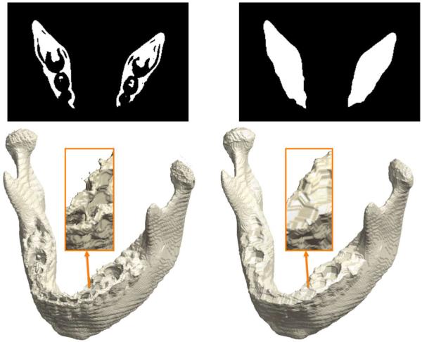
Image acquisition and processing artifacts and partial voluming produce topological defects such as holes and handles in any medical image. In mandibles CT images, unwanted cavities, holes and handles in the binary segmentation mainly result from differences in CT intensity between relatively low density mandible and teeth and more dense cortical bone and the interior trabecular bone (Andresen et al., 2000; Loubele et al., 2006). In mandibles, these topological noises can appear in thin or cancellous bone, such as in the condylar head and posterior palate (Stratemann et al., 2010). An example is shown in Figure 5, where the tooth cavity forms a bridge over the mandible. If we apply the isosurface extraction on the topologically defective segmentation results, the resulting surface will have many tiny handles (Wood et al., 2004; Yotter et al., 2009). These handles complicate subsequent surface mesh operations such as smoothing and parameterization. It is thus necessary to correct the topology by filling the holes and removing handles. If we correct such topological defects, it is expected that the resulting isosurface is topologically equivalent to a sphere.

Figure 5.

Topological correction on mandible binary segmentation and surface. Disjointed tiny speckles of noisy components are removed by labeling the largest connected component, and holes and handles are removed by the morphological closing operation. Left: A slice shows holes and handles in teeth regions. The isosurface has Euler characteristic χ = 50. Right: After the correction with χ = 2.

Various topology correction techniques have been proposed in medical image processing. Rather than attempting to repair the topological defects of the already extracted surfaces (Wood et al., 2004; Yotter et al., 2009), we performed the topological simplification on the volume representation directly using morphological operations (Guskov and Wood, 2001; Van Den Boomgaard and Van Balen, 1992; Yotter et al., 2009). The direct correction on surface meshes can possibly cause surfaces to intersect each other (Wood et al., 2004). By checking the Euler characteristic, the holes were automatically filled up using morphological operations to make the mandible binary volume topologically equivalent to a solid sphere. All areas enclosed by the higher density bone included in the mandible definition are morphed into being in the definition of the mandible object. The hole-filled images were then converted to surface meshes via the marching cubes algorithm.

In our fully automated algorithm, we first removed the speckles of noise components by identifying the largest connected component in the binary volume. Then we applied the morphological closing operation in each 2D slice of CT images one by one in all three axes. Recombining the topology-corrected 2D slices resulted in topologically correct surface meshes (Figure 5). 2D topological closing operations were used mainly due to its performance and relatively simpler implementation than 3D topological closing operations. In 2D topological operations, we only to consider only 8 neighboring voxels in a 2D image slice compared to 26 neighboring voxels in a 3D image volume. There are many large concave regions left out by teeth and fillings. These regions may not be closed with 3D closing operations but can be easily patched up with 2D closing operations, which tend to put more constraints on the underlying topology. Instead of performing a single 3D closing operation that may not work, we sequentially performed 2D closing operations in each image slice in all the x-, y- and z-directions. Figure 6 shows a simulated cavity example that was not patched by existing 3D closing operation (Van Den Boomgaard and Van Balen, 1992) but was easily patched by the sequential application of 2D closing operations. Note that any 3D object, whose every 2D cross-section is topologically equivalent to a solid disk, is topologically equivalent to a solid sphere. The problem of 3D topology correction can be thus reduced to a much simpler problem of 2D topology correction of multiple slices.

Figure 6.

Cavity patching by topological closing operations. Left: Surface model of the binary volume that simulates a tooth cavity. Middle: The 3D image volume based closing operation does not properly patch the cavity region. Right: The 2D image slice based closing operation patches the cavity region properly.

At the end of the processing, we checked the Euler characteristic of the resulting surface meshes. Note that for each triangle, there are three edges. For a closed surface topologically equivalent to a sphere, two adjacent triangles share the same edge. The total number of edges is thus E = 3F/2. We checked if the Euler characteristic is simply given by χ = V −F/2 at the end. All binary volumes produced the topologically correct surfaces without exception. Figure 5 shows an example of before and after the topology correction.

3.2. Validation and Performance Analysis of Heat Kernel Smoothing

Here, we compared the performance of the proposed kernel regression against iterated kernel and diffusion smoothing techniques. The high accuracy of the heat kernel construction using LB-eigenfunctions was reported in Kim et al. (2011).

3.2.1. Comparison against iterated kernel smoothing

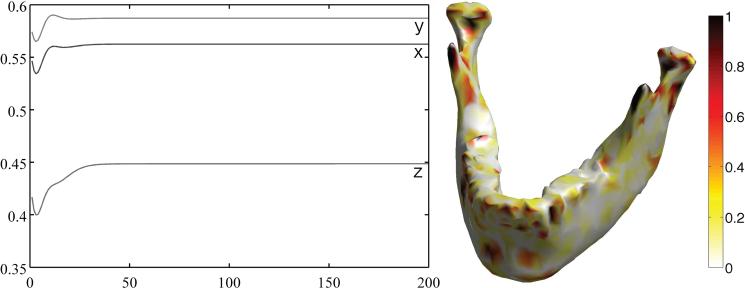
The proposed heat kernel regression was compared against the widely used iterated kernel smoothing framework (Chung et al., 2005; Hagler Jr. et al., 2006; Han et al., 2006). The x, y and z surface coordinates are treated as functional measurements on the original surface and smoothed with both methods. For the comparison of performance between both smoothing methods, we calculated the root mean squared errors (RMSE) between them. The mean of the squared errors is taken over the surface. For the heat kernel regression, we used the bandwidth σ = 0.5 and eigenfunctions up to k = 132 degree. For iterated kernel smoothing, we varied the number of iterations 1 ≤ m ≤ 200 with the correspondingly smaller bandwidth 0.5/m having the effective bandwidth of 0.5. The performance of the iterated kernel smoothing depended on the number of iterations, as shown in the plot of RMSE of mesh coordinates over the number of iterations (Figure 7). The RMSE reached up to 0.5901 and did not decrease even when we increased the number of iterations. The right image in Figure 7 shows the squared difference between the two methods. The difference is mainly localized in high curvature areas, where the Gaussian kernel used in the iterated kernel smoothing fails to approximate the heat kernel. This comparison quantitatively demonstrates the limitation of iterated heat kernel smoothing, which does not converge to heat diffusion.

Figure 7.

Plot of the RMSE of iterated kernel smoothing against the proposed heat kernel regression for coordinates x (middle), y (top) and z (bottom) over the number of iterations up to 200. For heat kernel regression, σ = 0.5 and k = 132 are used. Iterated kernel smoothing does not converge to heat diffusion. The right figure shows the squared difference between the two methods. The difference is mainly localized in high curvature areas, where the Gaussian kernel used in the iterated kernel smoothing fails to approximate the heat kernel.

3.2.2. Comparison against diffusion smoothing

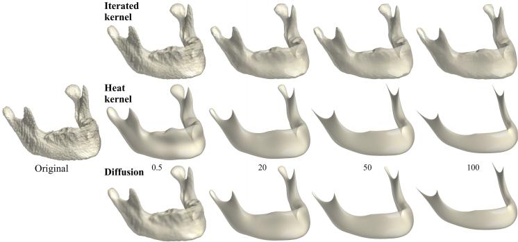
We further compared the proposed heat kernel regression to diffusion smoothing widely used in smoothing surface data (Chung et al., 2001; Andrade et al., 2001; Cachia et al., 2003a,b; Chung and Taylor, 2004). For the forward Euler scheme (6) to converge, we need to have sufficiently small step size Δσ. We investigated the convergence of diffusion smoothing against heat kernel regression with bandwidths σ = 0.5, 20, 50, 100 and k = 132. For diffusion smoothing, small fixed step size of Δσ = 0.025 was used with m = 20, 800, 2000, 4000 iterations. The diffusion smoothing result was found to be inaccurate for less than 10 iterations, but it converged quickly to heat kernel smoothing as the number of iterations m increased, giving the compatible results.

Figure 8 shows the result of smoothing surface coordinates with three different techniques: iterated kernel smoothing (Chung et al., 2005), the proposed kernel regression and diffusion smoothing based on FEM discretization (Chung and Taylor, 2004). We replaced the original surface coordinates with smoothed ones for the final visualization. However, in the actual computation, we did not replace the original surface coordinates for the three methods. Iterated kernel smoothing compounds the discretization errors over iterations, so it does not converge to kernel regression and diffusion smoothing. Diffusion smoothing and heat kernel smoothing share the same FEM discretization and are expected to converge as the bandwidth increases.

Figure 8.

Smoothed mandible surfaces using three different techniques with the same bandwidths. They are all expected to be the solution of isotropic diffusion. The x, y and z surface coordinates are treated as functional measurements on the original surface and smoothed. The proposed heat kernel smoothing is done with various bandwidths, σ = 0.5, 20, 50, 100. Iterated kernel smoothing performs iterative kernel smoothing with heat kernel approximated linearly with Gaussian kernel (Chung et al., 2005). Diffusion smoothing directly solves the diffusion equation using the same FEM discretization (Chung and Taylor, 2004). Diffusion smoothing and heat kernel smoothing converge to each other as the bandwidth increases.

3.3. Simulation Studies

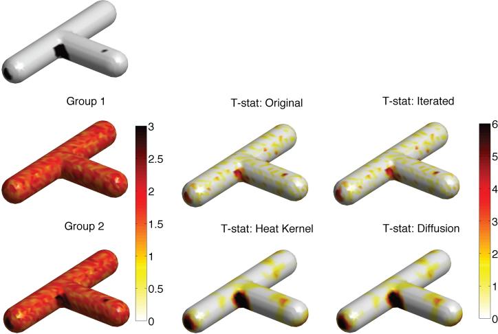
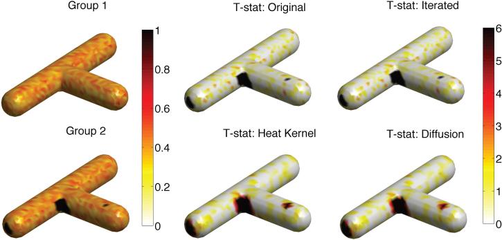
Since there is no known ground truth in the imaging data set we are using, it is uncertain how the proposed method will perform with the real data. It is therefore necessary to perform simulation studies with the ground truths. We performed two simulations with small and large signal-to-noise ratio (SNR) settings on a T-junction shaped surface (Figure 9). The T-junction surface was chosen because it was a surface with three different curvatures: convex, concave and almost flat regions. Note surface smoothing methods perform differently under different curvatures. Three black signal regions of different sizes were taken as the ground truth at these regions. 60 independent functional measurements on the T-junction were simulated as |N(0, γ²)|, the absolute value of normal distribution with mean and variance γ², at each mesh vertex. Value 1 was then added to the black regions in 30 of the measurements, which served as group 2, while the other 30 measurements were taken as group 1. Group 1 had distribution |N(0,γ²)| while group 2 had distribution |N(1,γ²)| in the signal regions. Larger variance γ² corresponds to smaller SNR. [notdef]

Figure 9.

Simulation study I on a T-junction shaped surface where three black signal regions of different sizes are taken as the ground truth. 60 independent functional measurements on the T-junction were simulated as |N(0, 2²)| at each mesh vertex. We are only simulating positive numbers to better reflect the positive measurements used in the study. Value 1 was added to the black regions in 30 of measurements which served as group 2 while the other 30 measurements were taken as group 1. T-statistics are shown for these simulation (original) and three techniques with bandwidth 0.5. Heat kernel smoothing performed the best in detecting the ground truth.

In Study I, γ² = 2² was used to simulate functional measurements with substantially smaller SNR. Figure 9 shows the simulation results. For iterated kernel and diffusion smoothing, we used bandwidth σ = 0.5 and 100 iterations. For smaller SNR, it is necessary to smooth with larger bandwidth, which is determined empirically. For heat kernel smoothing, the same bandwidth and 1000 eigenfunctions were used. The same number of eigenfunctions was used through out the study. For all three smoothing techniques, bandwidth is the main parameter that determines performance. The results are stable under the perturbation of other parameters. We then performed the two sample t-test with the random field theory based threshold of 4.90 to detect the group difference at 0.05 level.

Neither the raw data nor iterated smoothing were able to correctly identify any signal region. However, heat kernel and diffusion smoothing correctly identified 94% and 91% of the signal regions respectively. This improvement for heat kernel smoothing is significant considering that the error rate of 5% (α-level of 0.05) is considered as the standard threshold for accepting or rejecting a hypothesis. In addition heat kernel and diffusion smoothing incorrectly identified 0.26% and 0.26% of non-signal regions as signal. Although both methods use the similar FEM discretization schemes, diffusion smoothing suffers more discretization error. The discretization error is related to the forward Euler scheme that is often employed in diffusion smoothing (Chung, 2001; Andrade et al., 2001; Cachia et al., 2003b). For better accuracy, extremely small time steps are required but this requires a very large number of iterations, which slows the method drastically. There might be a more accurate faster discretization scheme but the proposed method is validated against existing standard methods in the medical imaging literature.

In Study II, γ² = 0.5² was used to simulate functional measurements with substantially larger SNR. Due to the large SNR, the group means showed visible group separations (Figure 10). For iterated kernel and diffusion smoothing, we used bandwidth σ = 0.1 and 100 iterations. For heat kernel smoothing, the same bandwidth and 1000 eigenfunctions were used. All the methods detected the signal regions; however, the heat kernel smoothing and diffusion smoothing techniques were more sensitive at large SNR. All the methods correctly identified the signal regions with 100% accuracy. The raw data and iterated kernel smoothing did not incorrectly identified any non-signal regions as signal. However, due to the blurring effects, heat kernel and diffusion smoothing incorrectly identified 0.9% and 0.8% non-signal regions as signal, which is negligible. For large SNR setting, all the methods were reasonably able to detect the correct signal regions with minimal error.

Figure 10.

Simulation study II on a T-junction shaped surface with the same ground truth as simulation study I (Figure 9). 60 independent functional measurements on the T-junction were simulated as |N(0, 0.5²)| at each mesh vertex. Value 1 was added to the black regions in 30 of the measurements, which served as group 2, while the remaining 30 measurements are taken as group 1. Due to large SNR, the group means show visible group separations. All the methods detected the signal regions; however, the heat kernel smoothing and diffusion smoothing techniques were more sensitive at large SNR.

In summary, in larger SNR, all three methods performed well. However, in substantially smaller SNR, the proposed kernel regression performed best, closely followed by diffusion smoothing. Neither the raw data nor iterated kernel smoothing performed well in the low SNR setting.

4. Application: Mandible Growth Analysis

As an illustration of the proposed kernel regression technique, we performed a mandible growth analysis on a CT imaging data set consisting of 77 human subjects between the ages of 0 and 19 years. Subjects were divided into three age categories: 0 to 6 years (group I, 26 subjects), 7 to 12 years (group II, 20 subjects), and 13 to 19 years (group III, 31 subjects). The main biological question of interest is whether there are localized regions of growth between these different age groups. Mandible surface meshes for all subjects were constructed through the image acquisition and processing steps described in the previous section. For surface alignment, diffeomorphic surface registration was used to match mandible surfaces across subjects (Miller and Qiu, 2009; Vaillant et al., 2007; Qiu and Miller, 2008; Yang et al., 2011).

4.1. Diffeomorphic Surface Registration

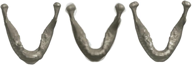
We chose the mandible of a 12-year-old subject identified as F155-12-08, which served as the reference template in previous studies (Seo et al., 2010, 2011), as initial template ${\mathcal{M}}_I$ and aligned the remaining 76 mandibles to the initial template a nely to remove the overall size variability. Some subject may have larger mandible than others so it is necessary to remove the global size differences in localized shape modeling. From the a ne transformed individual mandible surfaces ${\mathcal{M}}_j$, we performed an additional nonlinear surface registration to the template using the large deformation diffeomorphic metric mapping (LDDMM) framework (Miller and Qiu, 2009; Vaillant et al., 2007; Qiu and Miller, 2008; Yang et al., 2011).

In the LDDMM framework (Miller and Qiu, 2009; Vaillant et al., 2007; Qiu and Miller, 2008; Yang et al., 2011), given a surface $\mathcal{M}$, the metric space is constructed as an orbit of $\mathcal{M}$ under the group of diffeomorphic transformations $\mathcal{G}$, i.e. ${\mathcal{M}}_j=\mathcal{G}\cdot \mathcal{M}$ The diffeomorphic transformations (one-to-one, smooth forward and inverse transformation) are introduced as transformations of the coordinates on the background space $\Omega \subset {\mathbb{R}}^3$. The diffeomorphisms ${\varphi }_t\in \mathcal{G}$ are constructed as a flow of ordinary differential equations (ODE), where ϕ_t, t ∈ [0, 1] follows

$${\stackrel{.}{\varphi }}_t=v_t\left({\varphi }_t\right),{\varphi }_0=\mathrm{Id},t\in [0,1],$$ (22)

where Id denotes the identity map and v_t are the associated velocity vector fields. The vector fields v_t are constrained to be sufficiently smooth, so that (22) is integrable and generates diffeomorphic transformations over finite time. The smoothness is ensured by forcing v_t to lie in a smooth vector field V , which is modeled as a reproducing kernel Hilbert space with linear operator L associated with norm ${\Vert u\Vert }_V^2={\langle Lu,u\rangle }_2$ (Dupuis et al., 1998). The group of diffeomorphisms $\mathcal{G}\left(V\right)$ is then the solutions of (22) with the vector fields satisfying ${\int }_0^1{\Vert v_t\Vert }_{V}dt<\infty$.

Given the template surface $\mathcal{M}$ and an individual surface ${\mathcal{M}}_j$, the geodesic ϕ_t, t ∈ [0, 1], which lies in the manifold of diffeomorphisms and connects $\mathcal{M}$ and ${\mathcal{M}}_j$, is defined as

$${\varphi }_0=\mathrm{Id},{\varphi }_1\cdot \mathcal{M}={\mathcal{M}}_j.$$

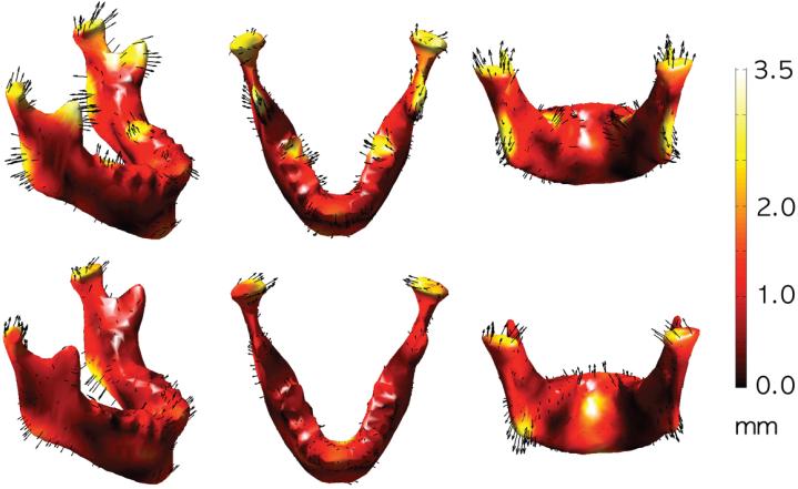
For our application, we employed the LDDMM approach to estimate the template among all subjects. The estimated template can be simply computed through averaging the initial velocity across all subjects (Zhong and Qiu, 2010), which is similar to the unbiased template estimation approach in Joshi et al. (2004). We then recomputed the displacement fields with respect to the initial template ${\mathcal{M}}_I$. We averaged the deformation fields from the initial template ${\mathcal{M}}_I$ to individual subjects to obtain the final template ${\mathcal{M}}_F$. Figure 11 shows the initial and final templates. Figure 12 shows the mean displacement differences between groups I and II (top) and II and III (bottom). Each row shows the group differences of the displacement: group II - group I (first row) and group III - group II (second row). The arrows are the growth direction with arrow length being representative of mean displacement differences and colors indicating growth length in mm.

Figure 11.

Left: Mandible F155-12-08, which forms an initial template ${\mathcal{M}}_I$. All other mandibles are a ne registered to F155-12-08. Middle: The superimposition of a ne registered mandibles showing local misalignment. Diffeomorphic registration is then performed to warp misaligned a ne transformed mandibles. Right: The average of deformation with respect to F155-12-08 provides the final population average template ${\mathcal{M}}_F$ where statistical parametric maps will be constructed.

Figure 12.

Mandibles were grouped into three age cohorts: group I (ages 0 to 6 years), group II (ages 7 to 12 years) and group III (ages 13 to 19 years). Each row shows the mean group differences of the displacement: group II - group I (first row) and group III - group II (second row). The arrows are the mean displacement differences and colors indicate their lengths in mm. Longer arrows imply more mean displacement.

4.2. Statistical Analysis

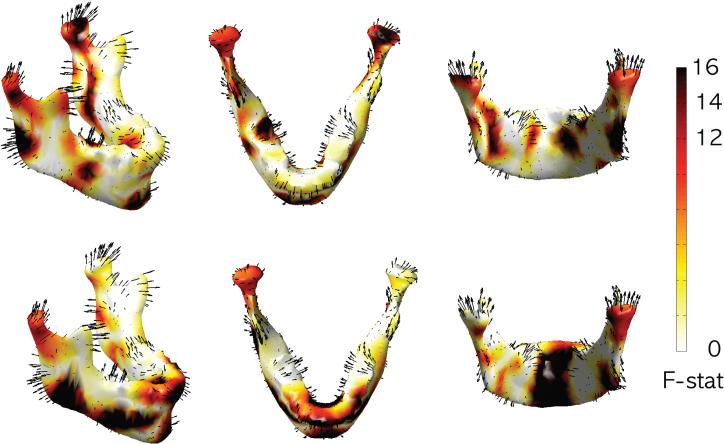
We are interested in determining the significance of the mean displacement differences in Figure 12. Since the length measurement provides a much easier biological interpretation, we used the length of the displacement vector as a response variable. The random field theory assumes the measurements to be smooth Gaussian random field. Heat kernel smoothing on the length measurement will make the length measurement smoother, more Gaussian and increase the signal-to-noise ratio (Chung et al., 2005). Heat kernel smoothing is applied with bandwidth σ = 20 using 1000 eigenfunctions on the final template ${\mathcal{M}}_F$. The number of eigenfunctions used is more than sufficient to guarantee a relative error less than 0.3%. The heat kernel smoothing of the displacement length is taken as the response variable. We constructed the F random field testing the length difference between the age groups I and II, and II and III showing the regions of accelerated growth (Figure 13).

Figure 13.

F -statistic map showing the regions of significant growth as measured by mean displacement difference between the groups displayed in Figure 12. The top row shows significant growth between groups I and II ; and bottom row between groups II and III.

For comparing the groups I and II, it is based on F -field with 1 and 44 degrees of freedom while for the groups II and III, it is based on F -field with 1 and 49. The multiple comparison corrected F -stat thresholds corresponding to α = 0.05 and 0.01 levels are respectively 8.00 and 10.52 (group II-I) and 8.00 and 10.67 (group III- II). In the F -statistic map shown in Figure 13, black and red regions are considered as exhibiting growth spurts at 0.01 and 0.05 levels respectively. Our findings are consistent with previous findings of simultaneous forward and downward growth (Scott, 1976; Smartt Jr. et al., 2005; Walker and Kowalski, 1972; Lewis et al., 1982; Seo et al., 2011) and bilateral growth (Enlow and Hans, 1996).

5. Conclusions

This study presents a novel heat kernel regression framework where the functional measurements are expanded using the weighted Laplace-Beltrami eigenfunctions analytically. The weighted eigenfunction expansion is related to isotropic heat diffusion and the diffusion wavelet transform. The method was validated on a unit sphere, where the spherical harmonics were the eigenfunctions. As demonstrated in the validation, the heat kernel regression provided more accurate results than the other surface-based smoothing techniques. Although both techniques share the identical FEM discretization, kernel regression is a parametric model while diffusion smoothing is not. The flexibility of the parametric model enabled to establish the mathematical equivalence of kernel regression, diffusion smoothing and diffusion wavelets.

The method was subsequently applied to characterize mandible growth. Based on the significant directions of the growth identified in Figure 12 and 13, we have quantified the regions, direction and extent of growth during periods in the first two decades of life that contribute towards the overall downward and forward growth of the mandible that has been described in the literature. For more comprehensive longitudinal growth modeling, we are currently securing additional samples.

References

- Adler R. The Geometry of Random Fields. John Wiley & Sons; 1981. [Google Scholar]
- Andrade A, Kherif F, Mangin J, Worsley K, Paradis A, Simon O, Dehaene S, Le Bihan D, Poline JB. Detection of fMRI activation using cortical surface mapping. Human Brain Mapping. 2001;12:79–93. doi: 10.1002/1097-0193(200102)12:2<79::AID-HBM1005>3.0.CO;2-I. [DOI] [PMC free article] [PubMed] [Google Scholar]
- Andresen PR, Bookstein FL, Conradsen K, Ersbøll BK, Marsh JL, Kreiborg S. Surface-bounded growth modeling applied to human mandibles. IEEE Transactions on Medical Imaging. 2000;19:1053–1063. doi: 10.1109/42.896780. [DOI] [PubMed] [Google Scholar]
- Antoine JP, Roşca D, Vandergheynst P. Wavelet transform on manifolds: old and new approaches. Applied and Computational Harmonic Analysis. 2010;28:189–202. [Google Scholar]
- Belkin M, Niyogi P, Sindhwani V. Manifold regularization: A geometric framework for learning from labeled and unlabeled examples. The Journal of Machine Learning Research. 2006;7:2399–2434. [Google Scholar]
- Bernal-Rusiel J, Atienza M, Cantero J. Detection of focal changes in human cortical thickness: spherical wavelets versus gaussian smoothing. NeuroImage. 2008;41:1278–1292. doi: 10.1016/j.neuroimage.2008.03.022. [DOI] [PubMed] [Google Scholar]
- Bronstein MM, Kokkinos I. Scale-invariant heat kernel signatures for non-rigid shape recognition. IEEE Conference on Computer Vision and Pattern Recognition (CVPR) 2010:1704–1711. [Google Scholar]
- Cachia A, Mangin JF, Riviére D, Kherif F, Boddaert N, Andrade A, Papadopoulos-Orfanos D, Poline JB, Bloch I, Zilbovicius M, Sonigo P, Brunelle F, Régis J. A primal sketch of the cortex mean curvature: a morphogenesis based approach to study the variability of the folding patterns. IEEE Transactions on Medical Imaging. 2003a;22:754–765. doi: 10.1109/TMI.2003.814781. [DOI] [PubMed] [Google Scholar]
- Cachia A, Mangin JF, Riviére D, Papadopoulos-Orfanos D, Kherif F, Bloch I, Régis J. A generic framework for parcellation of the cortical surface into gyri using geodesic Voronoï diagrams. Image Analysis. 2003b;7:403–416. doi: 10.1016/s1361-8415(03)00031-8. [DOI] [PubMed] [Google Scholar]
- Cao J, Worsley K. Applications of random fields in human brain mapping. Spatial Statistics: Methodological Aspects and Applications. 2001;159:170–182. [Google Scholar]
- Chung M. Ph.D. Thesis. McGill University; 2001. Statistical Morphometry in Neuroanatomy. http://www.stat.wisc.edu/~mchung/papers/thesis.pdf. [Google Scholar]
- Chung M, Hartley R, Dalton K, Davidson R. Encoding cortical surface by spherical harmonics. Statistica Sinica. 2008;18:1269–1291. [Google Scholar]
- Chung M, Robbins S, Evans A. Unified statistical approach to cortical thickness analysis. Information Processing in Medical Imaging (IPMI) Lecture Notes in Computer Science. 2005;3565:627–638. doi: 10.1007/11505730_52. [DOI] [PubMed] [Google Scholar]
- Chung M, Taylor J. Diffusion smoothing on brain surface via finite element method. Proceedings of IEEE International Symposium on Biomedical Imaging (ISBI) 2004:432–435. [Google Scholar]
- Chung M, Worsley K, Taylor J, Ramsay J, Robbins S, Evans A. Diffusion smoothing on the cortical surface. NeuroImage. 2001;13:S95. [Google Scholar]
- Coifman R, Maggioni M. Diffusion wavelets. Applied and Computational Harmonic Analysis. 2006;21:53–94. [Google Scholar]
- Dupuis P, Grenander U, Miller MI. Variational problems on flows of diffeomorphisms for image matching. Quarterly of Applied Math. 1998;56:587–600. [Google Scholar]
- Enlow DH, Hans MG. Essentials of Facial Growth. W.B. Saunders Company; Philadelphia: 1996. [Google Scholar]
- Evans L. Partial differential equations. American Mathematical Society; 1998. [Google Scholar]
- Gaser C, Luders E, Thompson P, Lee A, Dutton R, Geaga J, Hayashi K, Bellugi U, Galaburda A, Korenberg J, Mills D, Toga A, Reiss A. Increased local gyrification mapped in williams syndrome. NeuroImage. 2006;33:46–54. doi: 10.1016/j.neuroimage.2006.06.018. [DOI] [PubMed] [Google Scholar]
- de Goes F, Goldenstein S, Velho L. A hierarchical segmentation of articulated bodies. Computer Graphics Forum. 2008;27:1349–1356. [Google Scholar]
- Guskov I, Wood Z. Topological noise removal. Graphics Interface. 2001:19–26. [Google Scholar]
- Hagler D, Jr., Saygin A, Sereno M. Smoothing and cluster thresholding for cortical surface-based group analysis of fMRI data. NeuroImage. 2006;33:1093–1103. doi: 10.1016/j.neuroimage.2006.07.036. [DOI] [PMC free article] [PubMed] [Google Scholar]
- Hammond D, Vandergheynst P, Gribonval R. Wavelets on graphs via spectral graph theory. Applied and Computational Harmonic Analysis. 2011;30:129–150. [Google Scholar]
- Han J, Kim J, Chung C, Park K. Evaluation of smoothing in an iterative lp-norm minimization algorithm for surface-based source localization of meg. Physics in Medicine and Biology. 2007;52:4791–4803. doi: 10.1088/0031-9155/52/16/006. [DOI] [PubMed] [Google Scholar]
- Han X, Jovicich J, Salat D, van der Kouwe A, Quinn B, Czanner S, Busa E, Pacheco J, Albert M, Killiany R, et al. Reliability of MRI-derived measurements of human cerebral cortical thickness: The effects of field strength, scanner upgrade and manufacturer. NeuroImage. 2006;32:180–194. doi: 10.1016/j.neuroimage.2006.02.051. [DOI] [PubMed] [Google Scholar]
- Hernandez V, Roman JE, Tomas A, Vidal V. A Survey of Software for Sparse Eigenvalue Problems. Technical Report STR-6. Universidad Politécnica de Valencia. 2006 http://www.grycap.upv.es/slepc.
- Jo H, Lee JM, Kim JH, Shin YW, Kim IY, Kwon J, Kim S. Spatial accuracy of fmri activation influenced by volume- and surface-based spatial smoothing techniques. NeuroImage. 2007;34:550–564. doi: 10.1016/j.neuroimage.2006.09.047. [DOI] [PubMed] [Google Scholar]
- Joshi A, Shattuck DW, Thompson PM, Leahy RM. A parameterization-based numerical method for isotropic and anisotropic diffusion smoothing on non-flat surfaces. IEEE Transactions on Image Processing. 2009;18:1358–1365. doi: 10.1109/TIP.2009.2016163. [DOI] [PMC free article] [PubMed] [Google Scholar]
- Joshi SC, Davis B, Jomier M, Gerig G. Unbiased diffeomorphic atlas construction for computational anatomy. NeuroImage. 2004;23:151–160. doi: 10.1016/j.neuroimage.2004.07.068. [DOI] [PubMed] [Google Scholar]
- Kim SG, Chung M, Seo S, Schaefer S, van Reekum C, Davidson R. Heat kernel smoothing via Laplace-Beltrami eigenfunctions and its application to subcortical structure modeling, in: Pacific-Rim Symposium on Image and Video Technology (PSIVT). Lecture Notes in Computer Science (LNCS) 2011:36–47. [Google Scholar]
- Kim W, Pachauri D, Hatt C, Chung M, Johnson S, Singh V. Wavelet based multi-scale shape features on arbitrary surfaces for cortical thickness discrimination. Advances in Neural Information Processing Systems. 2012:1250–1258. [PMC free article] [PubMed] [Google Scholar]
- Lai Z, Hu J, Liu C, Taimouri V, Pai D, Zhu J, Xu J, Hua J. Intra-patient supine-prone colon registration in CT colonography using shape spectrum. Medical Image Computing and Computer-Assisted Intervention – MICCAI. 20102010:332–339. doi: 10.1007/978-3-642-15705-9_41. [DOI] [PubMed] [Google Scholar]
- Lehoucq R, Sorensen D, Yang C. ARPACK Users’ Guide: Solution of Large-Scale Eigenvalue Problems with Implicitly Restarted Arnoldi Methods. SIAM Publications; Philadelphia: 1998. [Google Scholar]
- Lerch JP, Evans A. Cortical thickness analysis examined through power analysis and a population simulation. NeuroImage. 2005;24:163–173. doi: 10.1016/j.neuroimage.2004.07.045. [DOI] [PubMed] [Google Scholar]
- Lévy B. Laplace-Beltrami eigenfunctions towards an algorithm that ”understands” geometry. IEEE International Conference on Shape Modeling and Applications. 2006:13. [Google Scholar]
- Lewis A, Roche A, Wagner B. Growth of the mandible during pubescence. The Angle Orthodontist. 1982;52:325–342. doi: 10.1043/0003-3219(1982)052<0325:GOTMDP>2.0.CO;2. [DOI] [PubMed] [Google Scholar]
- Loubele M, Maes F, Schutyser F, Marchal G, Jacobs R, Suetens P. Assessment of bone segmentation quality of cone-beam CT versus multislice spiral CT: a pilot study. Oral Surgery, Oral Medicine, Oral Pathology, Oral Radiology, and Endodontology. 2006;102:225–234. doi: 10.1016/j.tripleo.2005.10.039. [DOI] [PubMed] [Google Scholar]
- Luders E, Narr K, Thompson P, Rex D, Woods R, DeLuca H, Jancke L, Toga A. Gender effects on cortical thickness and the influence of scaling. Human Brain Mapping. 2006a;27:314–324. doi: 10.1002/hbm.20187. [DOI] [PMC free article] [PubMed] [Google Scholar]
- Luders E, Thompson P, Narr K, Toga A, Jancke L, Gaser C. A curvature-based approach to estimate local gyrification on the cortical surface. NeuroImage. 2006b;29:1224–1230. doi: 10.1016/j.neuroimage.2005.08.049. [DOI] [PubMed] [Google Scholar]
- Mahadevan S, Maggioni M. Value function approximation with diffusion wavelets and laplacian eigenfunctions. Advances in neural information processing systems. 2006;18:843. [Google Scholar]
- Malladi R, Ravve I. Fast difference schemes for edge enhancing Beltrami flow, in: Proceedings of Computer Vision-ECCV. Lecture Notes in Computer Science (LNCS) 2002:343–357. [Google Scholar]
- Miller M, Qiu A. The emerging discipline of computational functional anatomy. Neuroimage. 2009;45:S16–S39. doi: 10.1016/j.neuroimage.2008.10.044. [DOI] [PMC free article] [PubMed] [Google Scholar]
- Nain D, Styner M, Niethammer M, Levitt J, Shenton M, Gerig G, Bobick A, Tannenbaum A. Statistical shape analysis of brain structures using spherical wavelets. IEEE Symposium on Biomedical Imaging ISBI. 2007 doi: 10.1109/isbi.2007.356825. [DOI] [PMC free article] [PubMed] [Google Scholar]
- Niethammer M, Reuter M, Wolter F, Bouix S, Peinecke N, Koo M, Shenton M. Global Medical Shape Analysis Using the Laplace-Beltrami Spectrum. Lecture Notes in Computer Science. 2007;4791:850. doi: 10.1007/978-3-540-75757-3_103. [DOI] [PMC free article] [PubMed] [Google Scholar]
- Nilsson J, Sha F, Jordan M. Proceedings of the 24th international conference on Machine learning. ACM; 2007. Regression on manifolds using kernel dimension reduction; pp. 697–704. [Google Scholar]
- Perona P, Malik J. Scale-space and edge detection using anisotropic diffusion. IEEE Trans. Pattern Analysis and Machine Intelligence. 1990;12:629–639. [Google Scholar]
- Qiu A, Bitouk D, Miller M. Smooth functional and structural maps on the neocortex via orthonormal bases of the laplace-beltrami operator. IEEE Transactions on Medical Imaging. 2006;25:1296–1396. doi: 10.1109/tmi.2006.882143. [DOI] [PubMed] [Google Scholar]
- Qiu A, Miller M. Multi-structure network shape analysis via normal surface momentum maps. NeuroImage. 2008;42:1430–1438. doi: 10.1016/j.neuroimage.2008.04.257. [DOI] [PubMed] [Google Scholar]
- Reuter M. Hierarchical shape segmentation and registration via topological features of Laplace-Beltrami eigenfunctions. International Journal of Computer Vision. 2010;89:287–308. [Google Scholar]
- Reuter M, Wolter FE, Peinecke N. Laplace-Beltrami spectra as shape-dna of surfaces and solids. Computer-Aided Design. 2006;38:342–366. [Google Scholar]
- Reuter M, Wolter FE, Shenton M, Niethammer M. Laplace-Beltrami eigenvalues and topological features of eigenfunctions for statistical shape analysis. Computer-Aided Design. 2009;41:739–755. doi: 10.1016/j.cad.2009.02.007. [DOI] [PMC free article] [PubMed] [Google Scholar]
- Rosenberg S. The Laplacian on a Riemannian Manifold. Cambridge University Press; 1997. [Google Scholar]
- Rustamov R. Laplace-Beltrami eigenfunctions for deformation invariant shape representation. Proceedings of the fifth Eurographics symposium on Geometry processing. 2007:233. [Google Scholar]
- Schölkopf B, Smola AJ. Learning with Kernels: Support Vector Machines, Regularization, Optimization, and Beyond. MIT Press; 2002. [Google Scholar]
- Scott JH. Dento-facial Development and Growth. Pergamon Press; Oxford: 1976. [Google Scholar]
- Seo S, Chung M. Laplace-Beltrami eigenfunction expansion of cortical manifolds. Biomedical Imaging: From Nano to Macro; IEEE International Symposium on, IEEE.2011. 2011. pp. 372–375. [Google Scholar]
- Seo S, Chung M, Voperian H. Mandible shape modeling using the second eigenfunction of the laplace-beltrami operator. Proceedings of SPIE Medical Imaging. 2011:79620Z. [Google Scholar]
- Seo S, Chung M, Vorperian H. Heat kernel smothing using laplace-beltrami eigenfunctions. Medical Image Computing and Computer-Assisted Intervention – MICCAI. 20102010:505–512. doi: 10.1007/978-3-642-15711-0_63. [DOI] [PMC free article] [PubMed] [Google Scholar]
- Shawe-Taylor J, Cristianini N. Kernel methods for pattern analysis. Cambridge University Press; 2004. [Google Scholar]
- Shen L, Ford J, Makedon F, Saykin A. Surface-based approach for classification of 3d neuroanatomical structures. Intelligent Data Analysis. 2004;8:519–542. [Google Scholar]
- Shen L, Saykin A, Chung M, Huang H, Ford J, Makedon F, McHugh T, Rhodes C. Morphometric analysis of genetic variation in hippocampal shape in mild cognitive impairment: Role of an il-6 promoter polymorphism. Life Science Society Computational Systems Bioinformatics Conference. 2006 [Google Scholar]
- Shi Y, Dinov I, Toga AW. Cortical shape analysis in the Laplace-Beltrami feature space. 12th International Conference on Medical Image Computing and Computer Assisted Intervention (MICCAI 2009); 2009. pp. 208–215. [DOI] [PMC free article] [PubMed] [Google Scholar]
- Shi Y, Lai R, Kern K, Sicotte N, Dinov I, Toga AW. Harmonic surface mapping with Laplace-Beltrami eigenmaps. 11th International Conference on Medical Image Computing and Computer Assisted Intervention (MICCAI 2008); 2008. pp. 147–154. [DOI] [PMC free article] [PubMed] [Google Scholar]
- Smartt JM, Jr., Low DW, Bartlett SP. The pediatric mandible: I. A primer on growth and development. Plast. Reconstr. Surg. 2005;116:14e–23e. doi: 10.1097/01.prs.0000169940.69315.9c. [DOI] [PubMed] [Google Scholar]
- Sochen N, Kimmel R, Malladi R. A general framework for low level vision. IEEE Transactions on Image Processing. 1998;7:310–318. doi: 10.1109/83.661181. [DOI] [PubMed] [Google Scholar]
- Steinke F, Hein M. Non-parametric regression between manifolds. Advances in Neural Information Processing Systems . 2008 [Google Scholar]
- Stratemann SA, Huang JC, Maki K, Hatcher DC, Miller AJ. Evaluating the mandible with cone-beam computed tomography. American Journal of Orthodontics and Dentofacial Orthopedics. 2010;137:S58–S70. doi: 10.1016/j.ajodo.2009.01.025. [DOI] [PubMed] [Google Scholar]
- Styner M, Oguz I, Xu S, Brechbuhler C, Pantazis D, Levitt J, Shenton M, Gerig G. Framework for the statistical shape analysis of brain structures using spharm-pdm. Insight Journal, Special Edition on the Open Science Workshop at MICCAI. 2006 [PMC free article] [PubMed] [Google Scholar]
- Sun J, Ovsjanikov M, Guibas LJ. A concise and provably informative multi-scale signature based on heat diffusion. Comput. Graph. Forum. 2009;28:1383–1392. [Google Scholar]
- Tang B, Sapiro G, Caselles V. Direction diffusion. The Proceedings of the Seventh IEEE International Conference on Computer Vision. 1999:2, 1245–1252. [Google Scholar]
- Tasdizen T, Whitaker R, Burchard P, Osher S. Geometric surface smoothing via anisotropic diffusion of normals. Geometric Modeling and Processing. 2006:687–693. [Google Scholar]
- Taubin G. Geometric Signal Processing on Polygonal Meshes. EUROGRAPHICS. 2000 [Google Scholar]
- Taylor J, Worsley K. Detecting sparse signals in random fields, with an application to brain mapping. Journal of the American Statistical Association. 2007;102:913–928. [Google Scholar]
- Vaillant M, Qiu A, Glaunès J, Miller M. Diffeomorphic metric surface mapping in subregion of the superior temporal gyrus. NeuroImage. 2007;34:1149–1159. doi: 10.1016/j.neuroimage.2006.08.053. [DOI] [PMC free article] [PubMed] [Google Scholar]
- Vallet B, Lévy B. Spectral geometry processing with manifold harmonics. Computer Graphics Forum. 2008;27:251–260. [Google Scholar]
- Van Den Boomgaard R, Van Balen R. Methods for fast morphological image transforms using bitmapped binary images. CVGIP: Graphical Models and Image Processing. 1992;54:252–258. [Google Scholar]
- Walker GF, Kowalski CJ. On the growth of the mandible. American Journal of Physical Anthropology. 1972;36:111–118. doi: 10.1002/ajpa.1330360113. [DOI] [PubMed] [Google Scholar]
- Wang FY. Sharp explict lower bounds of heat kernels. Annals of Probability. 1997;24:1995–2006. [Google Scholar]
- Wang Y, Zhang J, Gutman B, Chan T, Becker J, Aizenstein H, Lopez O, Tamburo R, Toga A, Thompson P. Multivariate tensor-based morphometry on surfaces: Application to mapping ventricular abnormalities in HIV/AIDS. NeuroImage. 2010;49:2141–2157. doi: 10.1016/j.neuroimage.2009.10.086. [DOI] [PMC free article] [PubMed] [Google Scholar]
- Wardetzky M. Bobenko A, Sullivan J, Schröder P, Ziegler G, editors. Convergence of the cotangent formula: An overview. Discrete Differential Geometry. Birkhäuser Basel. volume 38 of Oberwolfach Seminars. 2008:275–286. [Google Scholar]
- Wood Z, Hoppe H, Desbrun M, Schröder P. Removing excess topology from isosurfaces. ACM Transactions on Graphics (TOG) 2004;23:190–208. [Google Scholar]
- Worlsey K, Poline JB, Vandal A, Friston K. Test for distributed, non-focal brain activations. NeuroImage. 1995;2:173–181. doi: 10.1006/nimg.1995.1024. [DOI] [PubMed] [Google Scholar]
- Worsley K. Detecting activation in fMRI data. Statistical Methods in Medical Research. 2003;12:401–418. doi: 10.1191/0962280203sm340ra. [DOI] [PubMed] [Google Scholar]
- Worsley K, Taylor J, Tomaiuolo F, Lerch J. Unified univariate and multivariate random field theory. NeuroImage. 2004;23:S189–195. doi: 10.1016/j.neuroimage.2004.07.026. [DOI] [PubMed] [Google Scholar]
- Yang X, Goh A, Qiu A. Locally linear diffeomorphic metric embedding (LLDME) for surface-based anatomical shape modeling. NeuroImage. 2011;56:149–161. doi: 10.1016/j.neuroimage.2011.01.069. [DOI] [PubMed] [Google Scholar]
- Yger F, Rakotomamonjy A. Wavelet kernel learning. Pattern Recognition. 2011;44:2614–2629. [Google Scholar]
- Yotter RA, Dahnke R, Gaser C. Medical Image Computing and Computer-Assisted Intervention (MICCAI) Springer; 2009. Topological correction of brain surface meshes using spherical harmonics; pp. 125–132. [DOI] [PubMed] [Google Scholar]
- Yushkevich P, Zhang H, Simon T, Gee J. Structure-specific statistical mapping of white matter tracts. NeuroImage. 2008;41:448–461. doi: 10.1016/j.neuroimage.2008.01.013. [DOI] [PMC free article] [PubMed] [Google Scholar]
- Zhang H, van Kaick O, Dyer R. Spectral methods for mesh processing and analysis. EUROGRAPHICS. 2007:1–22. [Google Scholar]
- Zhang H, van Kaick O, Dyer R. Spectral mesh processing. Computer Graphics Forum. 2010;29:1865–1894. [Google Scholar]
- Zhong J, Qiu A. Multi-manifold diffeomorphic metric mapping for aligning cortical hemispheric surfaces. Neuroimage. 2010;49:355–365. doi: 10.1016/j.neuroimage.2009.08.026. [DOI] [PubMed] [Google Scholar]
- Zhu H, Ibrahim J, Tang N, Rowe D, Hao X, Bansal R, Peterson B. A statistical analysis of brain morphology using wild bootstrapping. IEEE Transactions on Medical Imaging. 2007;26:954–966. doi: 10.1109/TMI.2007.897396. [DOI] [PMC free article] [PubMed] [Google Scholar]