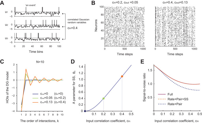
Figure 6. The ensemble activity simulated by the Dichotomized Gaussian (DG) model exhibits alternating signs of HOIs depending on successive orders of interaction.

(A) Illustration of a DG model of 3 neurons. The traces in each panel represent correlated input variables, at different time steps. The inputs are sampled from a multivariate Gaussian distribution, , with mean vector and covariance (See Methods). Here we assume that the mean vector contains the same scalar element, , in order to yield the activity probability , a value close to the empirically observed average activity rate (0.039 per 400 ms window). The off-diagonal elements of are all fixed at . The vertical lines above 0 in each panel mark the time steps at which an input crosses the threshold. (B) Simulation of the DG model with 100 neurons with weak (Left) and strong (Right) input correlations. The weak input correlation () in the Left panel yields a weak correlation coefficient () of output binary variables, whereas the strong input correlation () in the Right panel yields a stronger correlation coefficient () of output binary variables. (C) The HOIs of a small population from the DG model shows clear alternation of signs as the order of interaction increases except for . Negative interactions occur at odd and positive interactions occur at even . (D) The parameter of SS, , as a function of input correlation coefficient, . The dots marked in color represent at , 0.2, and 0.4. (E) The signal-to-noise ratio of the input correlation coefficient, , as a function of in the population activity of the DG model (The solid purple line). The dotted lines are signal-to-ratios in the subset features of the population activity (blue: the activity rates of individual and pairwise neurons; orange: the activity rates of individual and pairwise neurons plus the SS rate).