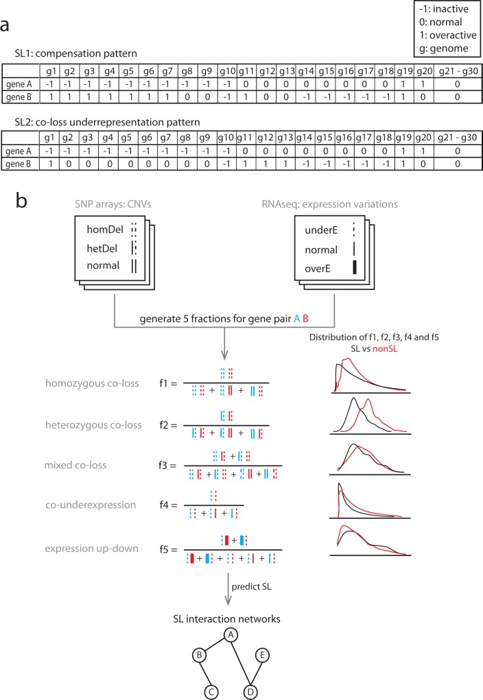
Fig 1. Patterns across cancer genomes reflecting selection against gene co-inactivation, and the workflow to predict SL interactions.

(a) A SL interaction SL1 between gene A and B can show a ‘compensation’ pattern across cancer genomes in which it is more likely that when A is inactive (denoted by -1), B is overactive (denoted by 1) to compensate the inactive A (genomes 1–10), compared to when A is active (genomes 11–30). SL interaction SL2 can, show a ‘co-loss underrepresentation’ in which a combined loss of A and B (denoted by -1 and -1, genome 10) across cancer genomes is underrepresented compared to a loss of either one of the two (genomes 2–9 and genome 14–18). Note that SL1 can also be identified via the co-loss underrepresentation pattern, but the SL2 can only be identified via the co-loss underrepresentation pattern. (b) The model requires two types of data as input, i) CNVs measured by SNP arrays and ii) gene expression variations measured by RNAseq. In CNVs, the status of a gene can be a homozygous deletion (two dash lines), a heterozygous deletion (one dash and one solid line) or normal (two solid lines). For CNVs, we generated three fractions to quantify the likelihood that a gene pair has a homozygous co-loss (f1), a heterozygous co-loss (f2) or a mixed co-loss (f3) event. In gene expression variations, a gene can be under-expressed (one dash line), normal (one solid line) or over-expressed (one bold line). For expression status, we generated two fractions, f4 and f5. f4 is the likelihood that both genes in a gene pair are under-expressed. f5 is the likelihood that a gene pair has an expression up-down event where one is over-expressed while the other one is under-expressed. All these five fractions showed a distribution difference between SL and non-SL pairs. By integrating these five fractions into a prediction model, we can identify SL interactions that can be presented as a network.