Figure 3.

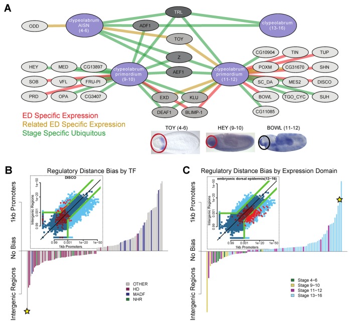
Applications of TF–domain association discovery. (A) Clypeolabrum network (66) example. Four expression gene sets from BDGP related to clypeolabrum development in the early embryo are shown as blue nodes ordered counter clockwise from the top left. Grey nodes indicate TFs. Edges are drawn when the corresponding TF–domain association is significant (<1E−7). TF nodes are colored from light to dark by the number of association edges they have. Edges are colored by the type of expression support indicated in the legend and have been filtered to remove TFs with similar motifs (SM9). TFs are clustered by the set of clypeolabrum expression domains they regulate. Below the network are in situ images of three different TFs at different stages whose clypeolabrum associations are supported with consistent expression. The clypeolabrum (black circle) emerges from the procephalon (red circles). (B) Distribution across binding domains families for TFs with greatest regulatory region biases. Each bar represents a different TF colored by its DBD family and height indicting the statistical strength of the bias between the proximal ‘p1K’ regulatory region and the more distal, insulator defined ‘IG’ regulatory region. The starred transcription factor is shown in detail in the inset plot with the P-values of the two methods for all TF–domain pairs in blue and for the 195 DISCO–domain pairs in red. Only points outside of the green lines are considered to be significantly biased. (C) Distribution across stages for expression domains with the greatest regulatory bias. Same as (B) with inset plot showing 325 TF associations with embryonic dorsal epidermis (stage 13–16).