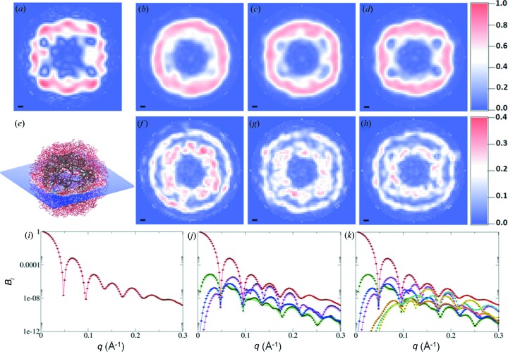
Figure 5.
Ab initio unconstrained shape reconstructions from model STMV data. The reconstructions were performed by including l = 0 (i.e. SAXS data) [parts (b), (f) and (i)], l ≤ 6 [parts (c), (g) and (j)] or l ≤ 12 [parts (d), (h) and (k)] in the B l refinement. The top row [parts (a)–(d)] depicts density slices through the centre of the virus (e). The reference density (a) shows significant detail in the core of the virus, which is largely absent when only SAXS data are used (b) but which is reproduced, with increasing quality, when terms up to l = 6 (c) and l = 12 (d) are considered. Another striking improvement is the distinctly non-spherical outer boundary of the particle when fluctuation scattering data are used. The second row [parts (f)–(h)] displays the associated standard deviations in the electron density as obtained from the ten independent aligned reconstructions. The black bar [parts (a)–(d) and (f)–(h) represents 10 Å. The bottom row [parts (i)–(k)] shows the agreement between the data (black circles) and the MOSA-refined (multi-objective simulated annealing; see Appendix A) expansion coefficients [B 0(q) red, B 2(q) green, B 4(q) blue, B 6(q) magenta, B 8(q) orange, B 10(q) cyan and B 12(q) yellow] for SAXS [part (i)] and for fluctuation scattering [parts (j)–(k)]. The error bars represent the standard deviation from the ten reconstructions.

