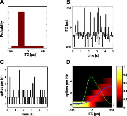
Fig. 2.

Computation of tuning curves and Fisher information (FI) from neural responses. A: each distribution of ITDs comprises a high-probability region (HPR) from which 80% of values are drawn, the remaining 20% contained within the range encompassed by the guinea pig's physiological range (±330 μs). Here the HPR is centered at −132 μs (i.e., leading in time at the ipsilateral ear) with a width of ± 66 μs. B: identical broadband noise (5 s) was presented to each ear with ITDs selected randomly every 50 ms from the distribution. C: the stimulus modulated the responses of isolated ITD-sensitive neurons (here in the form of a peristimulus time histogram). D: probability density function (pdf) of the response to multiple presentations of the HPR stimulus. The color indicates the probability of a particular spike count (number of spikes over a 50-ms epoch, on the y-axis) occurring in response to the ITD given on the x-axis (or, to be precise, the range of ITDs in an ∼13-μs bin). All presentations of the most negative (ipsilateral-leading) ITD, for example, evoked zero spikes, and therefore all spike counts for this ITD fall into the “0” bin. For increasingly contralateral ITDs, however, the proportion of trials evoking spikes increases, and thus the probability of spike counts occurring in bins other than “0” also increases. Note that as the spike count probability increases the variability of the spike count also increases (indicated by the spread of bins in which spike counts were observed). The spike count vs. ITD function is shown by the blue curve and the calculated FI by the green curve. The FI depends on both the mean of the spike count and its variability.