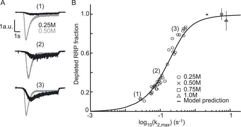
Figure 4. Relation between depleted RRP fraction and release kinetics.

(A) Examples of submaximal responses in different cells. 0.25M responses (black), scaled to 0.5M responses (grey) in the same cell, display faster kinetics when a larger fraction of the RRP is depleted. (B) Fitted data overlayed on the predicted curve. Data points corresponding to the examples in A are indicated. Data points for 0.50M, 0.75M, and 1.0M are shown as mean ± SEM. Note that whereas the model predicts a 94% depletion of the RRP with 0.5M the y-axis value at 0.5M is one per definition since the RRP size at this concentration was used as a reference to calculate the depleted RRP fraction.

DOI: http://dx.doi.org/10.7554/eLife.05531.017

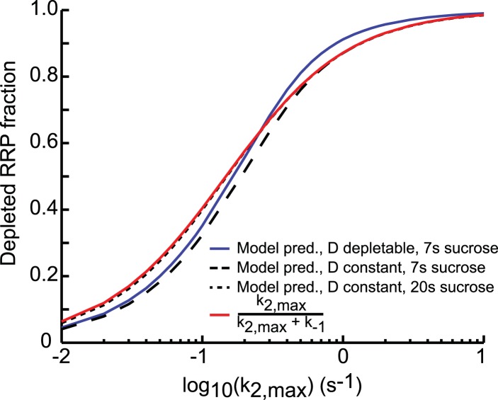
Figure 4—figure supplement 1. Comparison of analytical approximation and model predictions of the relation between release kinetics and RRP depletion.

For small k_2,max, the duration of the sucrose pulse dictates the depleted RRP fraction: 7 s stimuli deplete a smaller fraction than stimuli of 20 s and longer. For large k_2,max, the blue curve (D depletable) exceeds the others, because the steady-state RRP at the end of the stimulus is smaller when D is depletable. This is due to Equation (24): R_f = k₁D_f/(k₋₁ + k_2,max). A smaller upstream pool at the end of the stimulus (D_f) thus yields a smaller R_f and hence a larger depleted RRP fraction (R_i − R_f)/R_i.

DOI: http://dx.doi.org/10.7554/eLife.05531.019