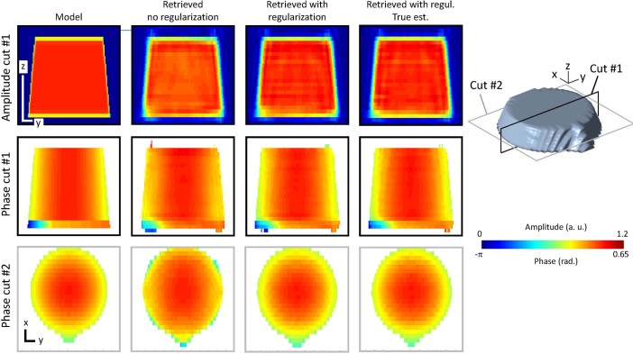
Figure 5. Optimizing the inversion scheme.

(Left) The 3D synthetic model object used to test the inversion procedure. It corresponds to the model shown on the right column of Figure 4. (Second column) Retrieved image using a conjugate gradient optimization of the Bouman and Sauer maximum likelihood, initialized with the shape of the object. (Third column) Same as before introducing an additional regularization term to constrain the sample support. (Right) Same as before, initialized with the true synthetic object. The top, middle and bottom rows are different cuts of the 3D object, as defined on the 3D isosurface plot rendition on the right. The assymetric spatial scale is given on left (y,z) and (x,y) cuts. Each line corresponds to a 100 nm length. The sample density and the displacement field color scales are indicated on the right. The excellent agreement observed between the two last retrieved solutions shows that the found inversion process is optimum.