Figure 3.

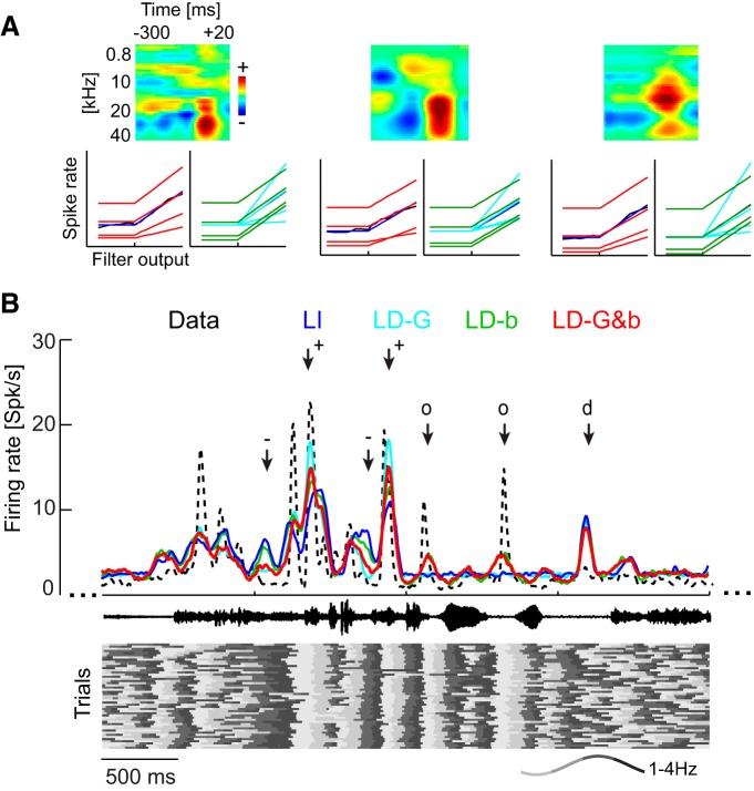
Example data from LNP models. A, Example data showing the STRFs and nonlinearities for three units. In the STRFs, red colors indicate time–frequency regions in which increases in acoustic energy drive firing rates and blue regions in which increases in energy reduce firing. The output nonlinearities are shown for the actual data (black) and each model. Note that the gain (slope) changes for the LD-G model (red), but it remains constant for the LD-b model (green). B, Example data showing the firing rate (trial averaged) for one unit for the actual data (black) and each model during acoustic stimulation. Responses were simulated on a single-trial basis. The sound waveform is indicated in the middle, and the bottom displays the delta phase (see example, wave for color code) in each trial that was used to shape the SD models. Arrows indicate periods of interest: +, periods in which LFP phase consistently across trials favors high gain and high background activity, and hence the LD models predict stronger responses than the LI model; −, periods in which LFP phase consistently favors low gain and background activity, and hence LD models predict a smaller response than the LI model; o, periods in which the stimulus filter (STRF) predicts no response (hence the LI response is flat) but LFP phase is consistently entrained to the stimulus and hence phase variations in background activity (LD-b, LD-G&b) predict changes in firing rates that coincide with those seen in the actual data; d, periods in which the LFP phase is not systematically aligned with the stimulus and all models predict very similar responses.