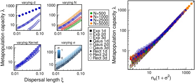
Fig 2. Dependence of the metapopulation capacity on various factors.

The four panels on the left show the metapopulation capacity λ vs. the dispersal length ξ. λ depends on the number of dimensions d (1, 2, 3), the number of patches N (500, 1000, 2500, 5000), the dispersal kernel f (Gaussian, Exponential and Rectangular), and the heterogeneity of patch value σ (varied between 0 and 1). Different symbols correspond to different combinations of f and d, while different colors correspond to different values of N. The color scale from blue to light blue refers to different values of σ. The right panel shows the collapsing of the various curves into a single one. The dependence on all the parameters (namely d, N, ξ, f and σ) is amalgamated in n _e(1+σ ²), where n _e is a simple function of all the parameters (computed via Monte Carlo integration, see S1 Text). The region of largest discrepancy (small n _e(1+σ ²)) corresponds to the localized case, where only few patches contribute to the persistence of the metapopulation (S1 Text). Without loss of generality, we set L = 1 in all simulations.