Children’s cognitive representation of the mathematical number line

Abstract

Learning of the mathematical number line has been hypothesized to be dependent on an inherent sense of approximate quantity. Children’s number line placements are predicted to conform to the underlying properties of this system; specifically, placements are exaggerated for small numerals and compressed for larger ones. Alternative hypotheses are based on proportional reasoning; specifically, numerals are placed relative to set anchors such as end points on the line. Traditional testing of these alternatives involves fitting group medians to corresponding regression models which assumes homogenous residuals and thus does not capture useful information from between- and within-child variation in placements across the number line. To more fully assess differential predictions, we developed a novel set of hierarchical statistical models that enable the simultaneous estimation of mean levels of and variation in performance, as well as developmental transitions. Using these techniques we fitted the number line placements of 224 children longitudinally assessed from first to fifth grade, inclusive. The compression pattern was evident in mean performance in first grade, but was the best fit for only 20% of first graders when the full range of variation in the data are modeled. Most first graders’ placements suggested use of end points, consistent with proportional reasoning. Developmental transition involved incorporation of a mid-point anchor, consistent with a modified proportional reasoning strategy. The methodology introduced here enables a more nuanced assessment of children’s number line representation and learning than any previous approaches and indicates that developmental improvement largely results from midpoint segmentation of the line.

Introduction

It is widely believed that a critical precursor for mathematical competence is the ability to mentally generate and understand the number line (Case & Okamoto, 1996). Indeed, children’s ability to accurately place numerals on the line is predictive of their later mathematics achievement, controlling other factors (Geary, 2011; Siegler & Booth, 2004). The nature of the cognitive systems that support children’s mental representation of the number line and the ordering of numerals on it, however, are vigorously debated (Ashcraft & Moore, 2012; Barth & Paladino, 2011; Cohen & Blanc-Goldhammer, 2011; Núñez, 2009; Núñez, Cooperrider & Wasserman, 2012; Slusser, Santiago, & Barth, 2013). One view is that humans have an inherent sense of approximate numerical magnitude that guides how children represent and order numerals on the number line (Ansari, 2008; Dehaene, 1997; Feigenson, Dehaene & Spelke, 2004; Gallistel & Gelman, 1992; Meck & Church, 1983). The ways in which this system represents magnitudes is debated as well (Dehaene, 2003; Gallistel & Gelman, 1992), but the result is the same: Smaller magnitudes are represented with greater precision than larger magnitudes.

Dehaene’s (1997, 2003) hypothesis that inherent representations of magnitudes are distinct for smaller quantities and increasingly compressed as magnitude increases has motivated many developmental studies of children’s number line learning (e.g. Ashcraft & Moore, 2012; Booth & Siegler, 2006; Geary, Hoard, Byrd-Craven, Nugent & Numtee, 2007). If the approximate system is organized in this way and if children directly map numerals onto these approximate magnitudes, then the pattern of number line placements will be compressed. Figure 1A provides an example of compressed placements – there is a tendency to overstate the magnitude for small numbers and understate the magnitude for larger ones. The exact form of the placement function follows a power law (Stevens, 1957).

Figure 1.

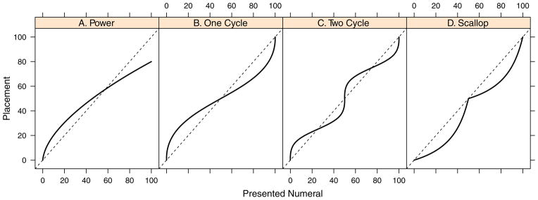
Four theoretical patterns of number placements. The solid lines denote mean placements.

An alternative is that the mapping of numerals onto the number line is based on proportional reasoning (Barth & Paladino, 2011; Cohen & Blanc-Goldhammer, 2011; Slusser et al., 2013). Across a wide range of tasks, including the estimation of proportional volume, area, and length, a strikingly similar pattern of findings have emerged. People show a systematic bias such that the magnitude of small proportions of a whole (e.g. a cylinder that is 10% full) are consistently overestimated, whereas the magnitude of larger proportions (e.g. a cylinder that is 90% full) are consistently underestimated (Hollands & Dyre, 2000; Spence, 1990; Spence & Krizel, 1994). These patterns seem to arise from the use of beginning and end (e.g. empty, full) anchors that result in perceptual biases and calibration of the to-be-judged information in relation to these anchors (Spence & Krizel, 1994). For instance, one of the biases referenced by Spence and Krizel is a contrast effect in which objects close to the anchor are judged further than veritical due to a center-surround contrastive mechanism. The proportional reasoning strategy explanation is attractive for tasks with clear anchors, and is particularly relevant for number line placements when the line has clearly marked beginning and end points. Accordingly, on a 0-to-100 number line, for instance, the numeral 25 is not directly mapped onto the line but is placed in reference to the 0 and 100 anchor points, in this case a quarter way between these points.

Figure 1B–D show various response patterns that have been interpreted as evidence for proportional reasoning. Figure 1B shows what is termed a one-cycle pattern (Hollands & Dyre, 2000; Spence, 1990; Spence & Krizel, 1994), and the key feature, as noted, is an overestimation of magnitudes for small numbers followed by an underestimation for larger ones. Figure 1C shows what is termed a two-cycle pattern (Hollands & Dyre, 2000) –the overestimation-then-underestimation pattern is repeated around the center point. This pattern is considered evidence for an additional anchor at the midpoint (Slusser et al., 2013), and may reflect the tendency for people to create a visual axis of symmetry where possible (Spence & Krizel, 1994). Figure 1D shows an alternative two-anchor proportional reasoning pattern, a scallop pattern. Cohen & Blanc-Goldhammer (2011) found such a pattern when adults made placements on a number line that only included an anchor at zero, that is, there was no presented end point anchor. We included this model to test all potential alternatives in the literature and because if children only use an anchor at zero when first learning the number line, their placements are conceptually unbounded as with the adults in Cohen and Blanc-Goldhammer’s study. In any case, the pattern in Figure 1D is also considered evidence for use of a midpoint anchor.

Figure 1 shows means or expected values. Consider an individual who makes repeated placements to a given numeral. The value in the figure at that numeral is the mean over these repeated placements. Yet, we need not be content to study the mean alone as for each presented numeral there is, at least hypothetically, a distribution of placements (Spence, 1990). As is frequently the case in cognitive psychology, the distribution is often more diagnostic for adjudicating between theories than the mean alone. The top row of Figure 2 shows the case when the variance of the distribution does not depend on the presented numeral, which is what is implicitly assumed when ordinary least squares (OLS) regression is used to fit placements. The five lines in each panel show the 10th, 30th, 50th (median), 70th and 90th percentiles of the placement distributions as a function of the presented numeral. When equal variances are assumed, the distances between the percentile lines are constant across the range of presented numerals. The figure makes clear the difference between variance and bias. Bias refers to how much distortion there is between the mean (or median) of the distribution and the true magnitude for the presented numeral. In Figure 2A, for example, there is an overestimation bias for small numerals and an underestimation bias for larger ones (see the middle line). In fact, the bias in each panel of Figure 2 matches the bias in the corresponding panels in Figure 1. Variance, in contrast, refers to spread around this mean, and is unrelated to bias. The top row of Figure 2 shows variances that do not change with the presented numeral even though the bias does.

Figure 2.

Contrasting models of the distribution of number line placements. The top row of plots shows the case when the four substantive patterns from Figure 1 are combined with the equal-variance assumption. The bottom row shows the case when the substantive models are combined with the distance-from-anchor variance assumption. The five lines in each plot correspond to predictions for the 10^th, 30^th, 50^th, 70^th, and 90^th percentiles.

The equal-variance assumption has two major drawbacks: First, it leads to infelicities such as predicting invalid placements below 0 and above 100. Second, and more importantly, the assumption is without psychological content. A better alternative is to use the theoretical positions themselves to inform assumptions about variance of the placement distributions. The bottom row of Figure 2 shows the logic. Figure 2E shows alternative hypothetical distributions for the compressed-scale model which is an amalgam of elements from Dehaene (1997, 2003) and Gallistel & Gelman (1992). The means here follow a power law, which is similar to Dehaene (1997, 2003), but the variances increase as well, as suggested by Gallistel & Gelman (1992). The increase in variance is seen by the increasing spread between the percentile lines.

The predictions for the proportional reasoning theory are based on a single principle – variation should be greater the further the number is from the nearest anchor. For the two-anchor models, those with anchor points at 0 and 100, the variance is smallest near these anchors and increasing far from them. Figure 2F provides an example of the corresponding one-cycle pattern with variance predictions. The median line still follows the typical one-cycle pattern with an overestimation for small numbers and an underestimation for larger ones. The variance, however, is smallest at the endpoints and largest in the middle of the range. Note here the difference between bias and variance. The peak biases are near numbers of 25 and 75, and there is no bias at 50. Nonetheless, the predicted variance is largest at 50. Figure 2G and 2H show distributional predictions that correspond to the two-cycle and scallop patterns, respectively. These patterns are considered evidence for three-anchor models with anchor points at 0, 50, and 100. Consequently, the variance is smallest at these anchors and greatest away from them, notably at the values of 25 and 75. Note that corresponding panels in the top and bottom rows have the same medians (and the same bias); the difference is solely in how variance changes with the presented numerals. It is the contrast between these figures that informs our modeling, presented next.

It is helpful to consider the principle that variability in placements increases with distance between the nearest bound. This principle is taken as axiomatic, perhaps almost as self-evident. The justification is that in this task children must calculate a distance between the presented numeral and the anchors, and then translate this distance into a physical distance to mark the line. The minimal requirement is that the variability in this physical distance is a function of the physical distance itself, which strikes us as reasonable. Such an assumption seems compatible with analog representations of numbers (Moyer & Landauer, 1967). In this case it is reasonable to expect that the variability of a distance estimate increases with the distance itself, much as estimating the distance between two poles increases as those poles become further apart. It is also compatible with propositional representations as well. Even if the mental distance between anchors and presented numerals is represented precisely in propositional format, which does not seem likely given the wealth of extant evidence, the translation to physical placements on the line is nonetheless noise prone. The notion that the noise in placement is increasing with the distance to the nearest physical anchor is realistic even if it describes only the translation between precise mental distances and realized physical ones.

Models

In this section we describe how the distributional models in the bottom row of Figure 2 are specified. We do so here for a single participant performing the task. Let x denote the presented numeral divided by 100, e.g. x = .5 corresponds to a presented numeral of 50. Let y denote the placement on the same scale, 0 ≤ y ≤ 1. Let x₁,x₂,…, x_N be a sequence of presented numerals for N trials, and let y₁,y₂,…,y_N be the resulting placements.

The compressed-scale model, denoted , is given by

$$log{y}_i=\alpha +\beta \times log{x}_i+{\epsilon }_i,$$ (1)

where ε_i is a zero-centered, normally distributed noise term with standard deviation σ. Parameters α and β are the power and scale, respectively. Figure 3a shows 24 randomly generated data points from a hypothetical individual that follows the compressed-scale model . The placements follow the compressed-scale curve, and the variance of the points increases with the presented numeral. Figure 3b shows the same data, but the axes are transformed so that the spacing follows a log function that compresses the larger numbers relative to the smaller ones. With this spacing on the axes, the data cluster around a straight line rather than a curve, and the variability around this line is constant. Note that Figures 3a and 3b show the same data – all that has changed are the axes. Model simply specifies this log scaling: the slope and intercept on the log space serve as parameters of interest, and the residuals on this space serve as an appropriate within-subject measure of variability. Individuals who are well fit by the compressed-scale model will differ in slope from one another and differ in intercept from one another. The variability of these slopes and intercepts across people serve as appropriate between-subjects measures of variability. Gallistel & Gelman’s (1992) compressed-scale model specifies veritical placements with increasing variance, and this pattern is implemented in when α = 0 and β = 1. Dehaene’s compressed scale model (1997) has compressed mean placements, which occurs when β < 1.¹

Figure 3.

The models capture differential variance predictions by specifying different transformations. The left column shows characteristic patterns and hypothetical data in the natural number space. The right column shows the data on transformed spaces that linearize the means and stabilize the variances. a. & b.: The compressed-scale model, . c. & d.: The two-anchor model, accounts for the one-cycle pattern. e.-g.: The three-anchor model, accounts for the two-cycle and scallop patterns.

Figure 1 shows patterns from two classes of proportional reasoning models: the one-cycle pattern which implicates a two-anchor model with anchors at the two endpoints, and the two-cycle and scallop patterns which implicate a three-anchor model with anchors at the two endpoints and a third at the midpoint. The two-anchor and three-anchor models are treated separately.

The two-anchor model, denoted , is given by

$$\varphi (y_i)=\alpha +\beta \times \varphi (x_i)+{\epsilon }_i,$$ (2)

where ϕ is the log-odds transform:

$$\varphi (x)=log\left(\frac{x}{1-x}\right).$$

Parameters α and β index bias. The one-cycle bias pattern in Figure 2F occurs when α = 0 and β < 1, and the reverse bias occurs (underestimation for small numerals and overestimation for larger ones) when α = 0 and β > 1. Parameter α indexes an overall bias; overall underestimation and overall overestimation occur for α < 0 and α > 0, respectively. A key property of the two-anchor model is that the error variance for numeral placements is greatest near 50, that is, those in the middle of the range, even if the responses are unbiased there. Figure 3C shows 24 hypothetical data points that follow a one-cycle bias pattern. Figure 3D shows the same data, except that in this plot the spacing on the axes follows the log-odds transform. This spacing expands the spacing at the end and compresses it near 50, far from the anchor. Consequently, this spacing linearizes the predictions, and, as before, variability on this space is a suitable measure of within-subject variability. The one-cycle pattern occurs when the slope on the transformed space is less than unity.

The three-anchor model which predicts both two-cycle and scallop patterns, denoted , is given by

$$\theta (y_i)=\alpha +\beta \times \theta (x_i)+{\epsilon }_I,$$ (3)

where θ is

$$\theta (x)=\{\begin{array}{cc}log\left(\frac{x}{.5-x}\right)& x<.5,\\ log\left(\frac{x-.5}{1-x}\right)& x\ge \mathrm{.5.}\end{array}$$

The function of paramaters α and β is analogous to that in the two-anchor model. The two-cycle pattern in Figure 3e occurs when α = 0 and β < 1; the scallop pattern in Figure 3g occurs when α < 0 and β = 1, and, moreover, the model can support a combination of two-cycle and scallop patterns. A key property of the three-anchor model is that variance is smallest at the anchors of 0, 50 and 100, and greatest away from the anchors, near 25 and 75. The spacings that linearize the patterns follow the transform θ, and these are shown in Figures 3f and 3h, respectively. Note how the two-cycle bias corresponds to a shallowed slope in the transformed space; scalloping corresponds to a change in intercept.

In summary, the pattern of variability in number line placements serves as a diagnostic feature: Gallistel & Gelman’s (1992) compression theories of number line representation predict larger variances in placements for larger numerals; proportional reasoning with two anchors at the endpoints predicts largest variances in placements for the middle of the range; and proportional reasoning models with three anchors predicts the largest variance in placements at one-quarter and three-quarters of the range. Previous researchers who used regression with its equal-variance assumptions are unable to capitalize on the differential predictions about variance shown in the bottom row of Figure 2. The differential predictions may be capitalized upon, however, by simultaneous consideration of within- and between-participant variation in these placements. We develop a set of novel hierarchical statistical models for this purpose. To understand the developmental trajectory of number representation in children, we used these models to analyze a unique longitudinal data set that includes the first to fifth grade, inclusive, number line placements of 224 children.

Method

The data are from a prospective longitudinal study of children’s mathematical development and risk of learning disability (Geary, 2011; Geary, Hoard, Nugent & Bailey, 2012). All kindergarten children from 12 elementary schools that serve families from a wide range of socioeconomic backgrounds were invited to participate. Parental consent and child assent were received for 37% (N = 311) of these children and 288 of them completed all or nearly all of the first year measures and one other child completed a subset of the measures. The current analyses are based on the 224 children (103 boys) who completed the number line task in first to fifth grade, inclusive.

Participants

The mean age at the time of the respective first and fifth grade assessments was 82 (SD = 4) and 133 (SD = 4) months. The racial composition was white (73%), Asian (5%), black (9%), and mixed race (8%), with the parents of the remaining children identifying them as Native American, Pacific Islander, or unknown. Across racial categories, 4% of the sample identified as ethnically Hispanic. Thirty-four percent of the children attending the schools from which the sample was drawn were eligible for free or reduced price lunches.

Number line estimation task

The stimuli were 24 25-cm number lines that included the 0 and 100 endpoints with a target number printed approximately 5 cm above it in a large font (72 pt). The target numbers were 3, 4, 6, 8, 12, 17, 21, 23, 25, 29, 33, 39, 43, 48, 52, 57, 61, 64, 72, 79, 81, 84, 90, and 96 (Siegler & Booth, 2004). Experimental stimuli were presented in a random order for each child.

After discussion about number lines and when it was determined that the child recognized the concept, a blank number line, containing only the endpoints 0 and 100, was presented and the child was asked to determine where the number 50 should go. The child was instructed to mark on the line where 50 should fall; a pencil-and-paper version was used in first grade and a computerized version, where the child used the mouse to mark the line, thereafter. A number line with the endpoints and the location of 50 marked was then shown to the child. To ensure that the child understood the task, the child’s response was compared to the presented version and the experimenter discussed with the child using sentences such as, ‘50 is half of 100, so it goes half way between 0 and 100’. The experimental trials were then administered, each beginning with the instruction, ‘this is zero (pointing) and this is 100 (pointing), where would the number go?’ There was no time constraint.

Procedure

The children were administered a group of experimental tasks in the fall of each grade and achievement tests in the spring of each grade. The number line task was administered along with the other experimental measures in the fall of first grade. To accommodate constraints on testing time, the task was moved to the spring assessments beginning in second grade.

Results

Figure 4 shows children’s placements on the 0-to-100 number line with marked endpoints. Each thin line corresponds to a single child’s placements. As can be seen, placements become substantially more accurate across the five-year span. Consideration of mean values (dark lines) in isolation might be interpreted as modest evidence for a transition from a compressed representation in first grade to use of a proportional reasoning strategy thereafter. As will be discussed next, this compressed representation interpretation for first graders is not supported by modeling the full set of data. Figure 5 provides a view of the size of errors – the average magnitude of errors is plotted as a function of the presented numeral. The critical feature is a dramatic dip near a stimulus-value of 50, indicating high accuracy and low variability in the middle of the range. Such a pattern is supportive of proportional reasoning with an anchor at the midpoint. The use of this anchor emerges for most students by second grade, and may serve as an early indicator of number line learning. Indeed, this trend is highly compatible with the following modeling results.

Figure 4.

Number placements for individuals (light gray lines). The blue line is the mean across participants.

Figure 5.

The magnitude of errors in placement as a function of grade level and presented numeral.

To better understand the developmental changes, we fit the power law models ( ), the two-anchor model ( ), and the three-anchor model ( ) that were described previously. This previous description, however, was for a single participant at a single wave rather than for multiple participants across multiple waves. The models were extended as hierarchical mixed models, and these extensions are provided in the Appendix. Our approach in assessment was to select the best model for each individual-by-grade combination and plot how the models fared across children and grades. The best fitting model was the one with the smallest root-mean-squared-error between observed and predicted placements; this approach is reasonable in this context because all three models had the same number of free parameters. Figure 6 shows how the best fitting models varied across grades. The size of the circle represents the number of children whose placements were best fit by the model noted on the y-axis. For example, 63% of first graders were best fit by the two-anchor proportional reasoning model. By second grade, a plurality of children were best fit by the three-anchor model. By fifth grade this three-anchor model provides the best representation of the placements for 58% of the children. The lines in the figure show individual transitions across grades, and the thickness of the line bundle shows the number of children who made the transition. As an example, the thick line from the two-anchor model in first grade to the three-anchor model in second grade shows the developmental point where many children begin using the midpoint as well as the endpoint anchors.

Figure 6.

Model-based results. The size of the circles correspond to the number of participants (out of 224) best accounted by a certain model. The lines show the numbers of participants that transition from one model to the next across the grades.

One surprising facet of the analysis is how poorly the compressed-scale model fared overall. It accounted for 20% of first graders’ placements and less than 9% of fifth graders’ placements. The relatively poor performance of the compressed-scale model in accounting for participants’ placements at the individual level serves as a point of contrast with the means in Figure 4 for first grade. This contrast highlights the advantage of modeling individuals’ placements rather than means or medians of placements across individuals.

To further assess the conclusion that the children’s placements were anchored by a midpoint, we plotted residuals for the 91% of fifth graders whose placements were best fit by either the two-anchor or three-anchor models (Figure 7). The residuals allow an opportunity to observe why models misfit – whether these reflect a missing anchor or unaccounted systematic distortion away from the anchors. The top plots show the residuals for individuals whose placements were best fit by the three-anchor model, and not surprisingly the residuals are smaller for this model (Panel b) than for the two-anchor model (Panel a). The misfit of the two-anchor model is in the middle of the range where the residuals tend to be systematically positive in value, indicating that the model systematically predicts placements that are too small. The critical residuals for testing the midpoint-anchor hypothesis are for the fifth graders whose placements were better fit by the two-anchor model. These are shown in Panels c and d, respectively. Although the residuals are of course smaller overall for the two-anchor model (it did indeed fit better overall), the model does not fit well at the middle of the range, where there is good fit for the three-anchor model. This pattern is compatible with the use of a mid-range anchor, and misspecification of the three-anchor model reflects misspecification of bias away from the anchors. The three-anchor model, therefore, captures the important structural property that proportional reasoning is occurring from a midpoint and endpoint anchors even though it may misspecify to a small degree mean placements away from the anchors for some participants.

Figure 7.

Residuals (observed placement -predicted placement) as a function of presented numeral for fifth-grade students. a & b. Residuals for the three-anchor and two-anchor models, respectively, for students who were better fit by the three-anchor model. c & d. Same for students who were better fit by the two-anchor models. The main pattern is smaller residuals in the middle of the range for the three-anchor model than the two-anchor model, indicating that there is a midpoint. This pattern holds even for participants whose data are better described by the two-anchor model.

Finally, we address the question of how mean placement values deviated from veridical in the three-anchor model. One precedented pattern, from Spence (1990) and Spence & Krizel (1994), is that the midpoint anchor will act much like a physical one. The resulting pattern should be the classic two-cycle pattern shown in Figure 1C. An alternative is the scallop pattern inspired by Cohen & Blanc-Goldenhammer (2011) shown in Figure 1D. Inspection of Figure 4, especially with regard the fifth graders, provides support for an overall underestimation concordant with the scallop pattern. The difference between the two-cycle and scallop patterns manifest in the intercept and slope in Model . The two-cycle pattern corresponds to slopes less-than-1 and no intercept; the scallop pattern corresponds to slopes around 1.0 and negative intercept. We examined parameters for the fifth grade students and found that almost all, 96%, had a negative intercept while slightly more than half, 55%, had slopes less than 1. The fact that almost all fifth graders had negative intercepts is interpreted as strong support for the relevance of the scallop pattern.

Discussion

Understanding children’s development of number-line representation is not only of practical importance, but helps to address more basic issues regarding how humans, and many non-human species, mentally represent numerical magnitude and how these representations are instantiated in the brain (Dehaene, 1997 2003; Gallistel & Gelman, 1992). The current analysis of a rich longitudinal data set with novel models that capture mean levels of performance, variation in performance, and developmental transitions provides for unique insights into how children mentally represent and operate on the mathematical number line, and complement recent cross-sectional studies that have assessed alternative models, albeit with more conventional statistical approaches, and developmental transitions (Slusser et al. 2013).

When analyzed with typical models that account for mean performance, our data are consistent with many other developmental studies: First graders’ mean performance was consistent with predictions from the compressed-scale model of magnitude representation and the across-grade means are consistent with the often observed shift from compressed placements to linear ones (Ashcraft & Moore, 2012; Geary et al., 2007; Geary, 2011; Siegler & Booth, 2004; Siegler & Opfer, 2003). The latter presumably reflects children’s learning of the linear structure of the number line.

The picture changes considerably when the data are modeled with custom mixed models that capture the full pattern of variation within and across children and grades. At this level, the majority of first graders’ placements were more consistent with the use of the two presented end points as anchors, and the placements of some of them were consistent with use of an additional midpoint anchor. The placements of these children are consistent with the proposal that number lines with marked endpoints can be solved as proportional reasoning problems (Barth & Paladino, 2011; Cohen & Blanc-Goldhammer, 2011; Hollands & Dyre, 2000). It is of course possible that first graders whose placements were best fit by the proportional reasoning models would have made placements consistent with the compression model in kindergarten. It is also possible that the compression pattern arises from use of 0 as a single anchor point, with the signature logarithmic pattern resulting from higher discrimination among numerals close to this single anchor and poorer discrimination among numerals most distant from this anchor, as suggested by Slusser et al. (2013).

Our most striking developmental finding is an early transition, say between the first and second grades, from a two-anchor model to a three-anchor model, with the third anchor being at the midpoint. It is possible that the single practice trial in which children were presented ‘50’ and asked to place it facilitated the use of the midpoint anchor. But studies that have not used 50 (or other midpoints) to explain the task have found the same pattern of early usage of endpoint anchors and across-grade transitioning to use of an additional midpoint anchor, as we found here (Barth & Paladino, 2011; Slusser et al., 2013). Moreover, the placements of the majority of first graders were not consistent with use of a midpoint anchor, suggesting that if our procedure facilitated use of such an anchor it only occurred after children understood the utility of this anchor in making their placements more accurate. Spence & Krizel (1994) in fact argued that children will use the axis of symmetry (midpoint) as a virtual anchor in many different types of proportional reasoning tasks (e.g. volume) and that older children use virtual anchors more frequently than younger children.

The compression model can be unified with the proportional reasoning models, and all of them can be understood in terms of placements guided by one, two, or three anchor points. The more anchors, the tighter the restrictions on where the presented numeral can be placed on the line. Developmental improvement then results from incorporation of additional anchors, one at a time, that partition the line into segments. Placements are made within these segments, with numerals close to an anchor placed with greater accuracy than those farthest from an anchor.

A final question is whether children can further subdivide the number line with placement of more intermediate anchors, say at .25 and .75 of the line. In our data, we see no evidence of variance reduction around any other point other than the midpoint. We suspect there may be a general limit of one virtual anchor due to working memory constraints. Once children begin to use the mid-point anchor, further improvements in placement accuracy may represent improvement in the ability to calibrate individual placements from the two closest anchors, as suggested by Spence & Krizel (1994) for other proportional reasoning tasks.

Appendix

Models through are specified for a single participant performing in a single wave. The models may be expanded for multiple participants performing in multiple waves as follows: Let i = 1,…,24 index the trial number, j = 1,…,224, index the participant, and let k = 1,…,5 index the grade-level. The three models are extended as follows:

$$\begin{array}{l}{\mathcal{M}}_{1}log(y_{\mathit{ijk}})={\alpha }_{jk}+{\beta }_{jk}log(x_{\mathit{ijk}})+{\epsilon }_{\mathit{ijk}},\\ {\mathcal{M}}_2\varphi (y_{\mathit{ijk}})={\alpha }_{jk}+{\beta }_{jk}\varphi (x_{\mathit{ijk}})+{\epsilon }_{\mathit{ijk}},\\ {\mathcal{M}}_3\theta (y_{\mathit{ijk}})={\alpha }_{jk}+{\beta }_{jk}\theta (x_{\mathit{ijk}})+{\epsilon }_{\mathit{ijk}},\end{array}$$

where for each model

$${\epsilon }_{\mathit{ijk}}\mid {\sigma }_{jk}^2~\text{Normal}(0,{\sigma }_{jk}^2).$$

Models through are linear regression models conveniently analyzed with Bayesian methods (Gelman, Carlin, Stern, & Rubin, 2004; Jackman, 2009). In Bayesian models, priors are needed for parameters. We use priors that are flexible and computationally convenient:

$$\begin{array}{l}{\alpha }_{jk}~\text{Normal}({\mu }_{\alpha },{\delta }_{\alpha })\\ {\beta }_{jk}~\text{Normal}({\mu }_{\beta },{\delta }_{\beta })\\ {\sigma }_{jk}^2=\text{Inverse}\text{Gamma}(3,2)\end{array}$$

Flat priors may be placed on μ_α and μ_β, and weakly informative inverse-gamma priors (shape of 3, scale of 2) are placed on δ_α and δ_β. These choices are termed the joint-effects prior, and this setup imparts minimal information. The resulting posteriors reflect in exceedingly large part the likelihood component from the data.

An alternative approach is to use hierarchical priors which share strength across individuals and grades. We have explored the following to smooth estimates:

$$\begin{array}{l}{\alpha }_{jk}~\text{Normal}({\eta }_{1_j}+{\eta }_{2_k},{\delta }_{\alpha })\\ {\beta }_{jk}~\text{Normal}({\gamma }_{1_j}+{\gamma }_{2_k},{\delta }_{\beta })\\ {\sigma }_{jk}^2={\tau }_{1_j}{\tau }_{2_k}\end{array}$$

where η_1j, γ_1j, and τ_1j describe the main effect of the jth participant on α_jk, β_jk, and ${\sigma }_{jk}^2$, respectively, and η_2k, γ_2k and τ_2k describe the same for the kth grade. We place flat (uninformed) priors on effect (η, γ), and weakly informative inverse gamma priors on variance scales τ₁ and τ₂ with a shape of 3.0 and a scale of 2.0. Both the priors lead to similar results as there are many trials per participant-by-grade combination. We report results here with the joint-effects prior because this setup is modestly less informative than the hierarchical prior.

There is a notable complication in fitting model , the three-anchor model. The model predicts that placements are between the two anchors nearest the presented numeral. That is, if the presented numeral is less than 50, then the predicted placement must be between 0 and 50. Likewise, if the presented numeral is greater than 50, then the predicted placement must be between 50 and 100, and if the presented numeral is exactly 50, then the placement must be exactly 50. If the data violate these constraints, then the model as stated is falsified. A reasonable fix is to allow the midpoint anchor to vary modestly around .5 from trial to trial, and such a model does not impose the above falsification constraints while preserving the patterns of placements shown in Figure 2D-F. We developed such a model, but analysis proved too computationally complicated. We were unable to develop efficient algorithms for the integration from conditional posterior distributions to marginal posterior distributions. As an alternative, we decided to ignore all placements that violate the above constraints in fitting model . These included 19% of placements in first grade, but this decreased considerably thereafter (5%, 2%, 2%, and 1% for second to fifth grade, respectively).

References

- Ansari D. Effects of development and enculturation on number representation in the brain. Nature Reviews: Neuroscience. 2008;9:278–291. doi: 10.1038/nrn2334. [DOI] [PubMed] [Google Scholar]
- Ashcraft MH, Moore AM. Cognitive processes of numerical estimation in children. Journal of Experimental Child Psychology. 2012;111:246–267. doi: 10.1016/j.jecp.2011.08.005. [DOI] [PubMed] [Google Scholar]
- Barth HC, Paladino AM. The development of numerical estimation:evidence against a representational shift. Developmental Science. 2011;14:125–135. doi: 10.1111/j.1467-7687.2010.00962.x. [DOI] [PubMed] [Google Scholar]
- Booth JL, Siegler RS. Developmental and individual differences in pure numerical estimation. Developmental Psychology. 2006;41:189–201. doi: 10.1037/0012-1649.41.6.189. [DOI] [PubMed] [Google Scholar]
- Case R, Okamoto Y. The role of central conceptual structures in the development of childrens thought. Monographs of the Society for Research in Child Development. 1996;61(1–2 Serial No 246) doi: 10.1111/j.1540-5834.1996.tb00536.x. [DOI] [PubMed] [Google Scholar]
- Cohen DJ, Blanc-Goldhammer D. Numerical bias in bounded and unbounded number line tasks. Psychonomic Bulletin & Review. 2011;18:331–338. doi: 10.3758/s13423-011-0059-z. [DOI] [PMC free article] [PubMed] [Google Scholar]
- Dehaene S. The number sense: How the mind creates mathematics. New York: Oxford University Press; 1997. [Google Scholar]
- Dehaene S. The neural basis of the Weber-Feechner law: a logarithmic mental number line. Trends in Cognitive Sciences. 2003;7:145–147. doi: 10.1016/s1364-6613(03)00055-x. [DOI] [PubMed] [Google Scholar]
- Feigenson L, Dehaene S, Spelke E. Core systems of number. Trends in Cognitive Sciences. 2004;8:307–314. doi: 10.1016/j.tics.2004.05.002. [DOI] [PubMed] [Google Scholar]
- Gallistel CR, Gelman R. Preverbal and verbal counting and computation. Cognition. 1992;44:43–74. doi: 10.1016/0010-0277(92)90050-r. [DOI] [PubMed] [Google Scholar]
- Geary DC. Cognitive predictors of individual differences in achievement growth in mathematics: a five year longitudinal study. Developmental Psychology. 2011;47:1539–1552. doi: 10.1037/a0025510. [DOI] [PMC free article] [PubMed] [Google Scholar]
- Geary DC, Hoard MK, Byrd-Craven J, Nugent L, Numtee C. Cognitive mechanisms underlying achievement deficits in children with mathematical learning disability. Child Development. 2007;78:1343–1359. doi: 10.1111/j.1467-8624.2007.01069.x. [DOI] [PMC free article] [PubMed] [Google Scholar]
- Geary DC, Hoard MK, Nugent L, Bailey DH. Mathematical cognition deficits in children with learning disabilities and persistent low achievement: a five year prospective study. Journal of Educational Psychology. 2012;104:206–223. doi: 10.1037/a0025398. [DOI] [PMC free article] [PubMed] [Google Scholar]
- Gelman A, Carlin JB, Stern HS, Rubin DB. Bayesian data analysis. 2. London: Chapman and Hall; 2004. [Google Scholar]
- Hollands JG, Dyre BP. Bias in proportion judgments: The cyclical power model. Psychological Review. 2000;107:500–524. doi: 10.1037/0033-295x.107.3.500. [DOI] [PubMed] [Google Scholar]
- Jackman S. Bayesian analysis for the social sciences. Chichester: John Wiley & Sons; 2009. [Google Scholar]
- Meck WH, Church RM. A mode control model of counting and timing processes. Journal of Experimental Psychology: Animal Behavior Processes. 1983;9:320–334. [PubMed] [Google Scholar]
- Moyer RS, Landauer TK. Time required for judgements of numerical inequality. Nature. 1967;215:1519–1520. doi: 10.1038/2151519a0. [DOI] [PubMed] [Google Scholar]
- Núñez R. Numbers and arithmetic: neither hardwired ~ nor out there. Biological Theory. 2009;4:68–83. [Google Scholar]
- Núñez R, Cooperrider K, Wasserman J. Number concepts without number lines in an indigenous group of Papua NNew Guinea. PLoS ONE. 2012 doi: 10.1371/journal.pone.0035662. Retrieved from. [DOI] [PMC free article] [PubMed] [Google Scholar]
- Siegler RS, Booth JL. Development of numerical estimation in young children. Child Development. 2004;75:428–444. doi: 10.1111/j.1467-8624.2004.00684.x. [DOI] [PubMed] [Google Scholar]
- Siegler RS, Opfer JE. The development of numerical estimation: Evidence for multiple representations of numerical quantity. Psychological Science. 2003;14:237–243. doi: 10.1111/1467-9280.02438. [DOI] [PubMed] [Google Scholar]
- Slusser EB, Santiago RT, Barth HC. Developmental change in numerical estimation. Journal of Experimental Psychology: General. 2013;142:193–208. doi: 10.1037/a0028560. [DOI] [PubMed] [Google Scholar]
- Spence I. Visual psychophysics of simple graphical elements. Journal of Experimental Psychology: Human Perception and Performance. 1990;16:683–692. doi: 10.1037//0096-1523.16.4.683. [DOI] [PubMed] [Google Scholar]
- Spence I, Krizel P. Children’s perception of proportion in graphs. Child Development. 1994;65:1193–1213. [Google Scholar]
- Stevens SS. On the psychophysical law. Psychological Review. 1957;64:153–181. doi: 10.1037/h0046162. [DOI] [PubMed] [Google Scholar]