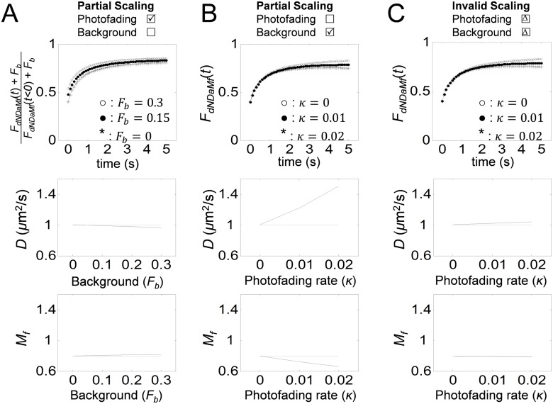
Fig 5. Analysis of the magnitude of errors caused by applying incompatible scaling or by using an incorrect sequence of scaling during FRAP analysis.
FRAP curves were simulated assuming D = 1μm2/s, F 0 = 0.4, F i = 1, r n = 1μm, and r e = 2μm under different scaling scenarios. Curves were then analyzed as indicated to obtain the best fits for D and M f. (A) FRAP curves were simulated using (f dNDaMf(t)+F b)/(f dNDaMf(t < 0)+F b) assuming κ = 0.005 s−1 and 0 ≤ F b ≤ 0.3 and then analyzed using f dNDaMf(t) (Eq 42) while ignoring F b. (B) FRAP curves were simulated using f dNDaMf(t) assuming M f = 0.8 and 0 ≤ κ ≤ 0.02 s−1 and then analyzed using f NDaMf(t) (Eq 37) while ignoring photofading. (C) FRAP curves were simulated using f dNDaMf(t) (Eq 42) assuming M f = 0.8 and 0 ≤ κ ≤ 0.02 s−1 and analyzed using an incorrectly scaled FRAP equation (Eq 44). Panels in the 2nd row show best fitting D as a function of variable conditions, F b and κ. Panels in the 3rd row show best fitting M f as a function of variable conditions, F b and κ.

