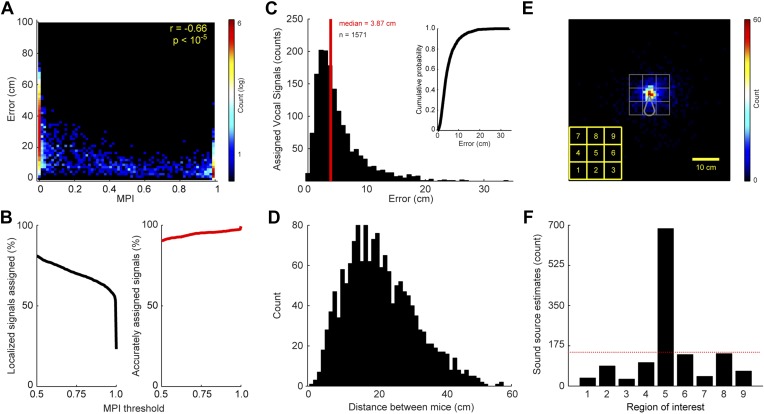
Figure 2. Accuracy and precision of sound-source localization system.
(A) Heat map shows inverse relationship between MPI and the distance between the mouse and estimated sound source location (r = -0.66; p < 10-5). The heat map is plotted in log counts with red indicating the maximum. Data for real and virtual mice are included in the plot. (B) Left panel shows the MPI threshold plotted relative to the percent of localized signals that were assigned. Right panel indicates the percentage of accurately assigned vocal signals plotted as a function of MPI threshold. (C) Distribution of the errors between the location of the estimated sound source and real source for assigned vocalizations. Median error is plotted in red. Inset shows the cumulative probability histogram of the errors. (D) Distribution of distances between the mouse assigned the vocalization and the animal closest to the assigned mouse. (E) Heat map showing sound source estimates (n = 2590) relative to mouse position (nose shifted to origin and rotated upwards). Gray sector shows mouse body. The large gray square, which is divided into smaller squares, indicates the regions of interest used to determine the precision of sound source localization system. Yellow key located at the bottom left indicates numbering scheme for smaller regions of interest. (F) Bar plot showing the number of sound source localization estimates in each of the smaller regions of interest. Region 5 includes the head of the mouse. Red line shows the expected counts based on a uniform distribution. The distribution of predicted sound source locations was significantly different between regions ( = 2305.7, p < 10−5).

