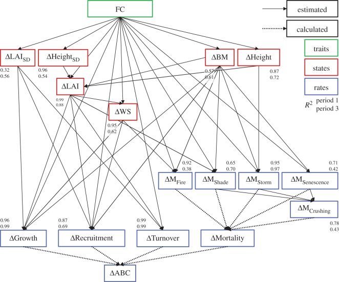
Figure 4.

Path model used to analyse the effect paths of FC on the target variable ΔABC (biodiversity effect in ABC) via intermediate states and rates. All states and rates represent the biodiversity effect in them (difference between observation and null model expectation), denoted by a leading Δ. Solid lines were estimated with linear regressions as part of the path modelling. Dotted lines were calculated, such that ΔABC was the sum of ΔGrowth, ΔRecruitment, ΔTurnover (leaf and roots) and ΔMortality and ΔMortality was the sum of five mortality processes. The model fits (R²) are placed directly adjacent to the estimated variables with the model fit for period 1 above and period 3 below. FC comprises functional richness, functional dissimilarity and functional identity. States are BM, biomass (kg C m⁻²); Height, tree height (m); LAI, leaf area index (m²/m²); LAI_SD, the standard deviation of LAI across patches and years in a time period, Height_SD the standard deviation of Height in a patch and WS, a metric between 0 and 1 indicating water stress. Rates (kg C m⁻² yr⁻¹): ABC, annual biomass change; Growth, growth of existing trees; Recruitment, growth of new regeneration; Turnover, turnover of roots and leaves; Mortality, mortality of living trees; M, mortality due to five processes: Shade, Senescence, Storm, Fire and Crushing. We analysed the biodiversity effect on states and rates, indicated by a leading Δ. Where applicable, we used averages weighted by tree and/or patch biomass. This figure omits some intermediate rates (such as e.g. NPP) that are not discussed in this paper, but see electronic supplementary material, Figure C1 in Appendix C.