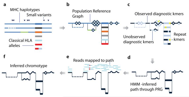
Figure 2. Schematic illustration showing the construction and application of a population reference graph.

a. Multiple sources of information about genetic variation, including alternative reference haplotypes (lines), classical HLA alleles (rectangles) and SNPs / short indels (triangles) are aligned. Colours indicate divergent sequence, dashes indicate gaps. b. A population reference graph (PRG) is constructed from the alignment, resulting in a generative model for variation within the region. SNPs, indicated by diamonds, are added as alternative paths to all valid backgrounds (i.e. excluding sequence with gaps or a third allele at the position). c. The PRG is compared to the de Bruijn graph constructed from reads obtained from a sample. Informative kmers (i.e. those that are found at only one level in the PRG) are identified (dark blue). Those found elsewhere in the genome (yellow) are ignored. d. A hidden Markov model is used to infer the most likely pair of paths through the PRG, allowing for read errors, resulting in an individualized reference chromotype for the sample. e. Two haploid genomes are constructed from the reference chromotype, with arbitrary phasing between adjacent bubbles, and reads (light blue lines) from the sample are aligned and assigned (on the basis of mapping quality) to a reference, thus identifying places where the sample contains novel variation (red circles; only one path through the chromotype is shown). f. Newly-discovered variants modify the reference chromotype, resulting in the inferred chromotype for the sample.