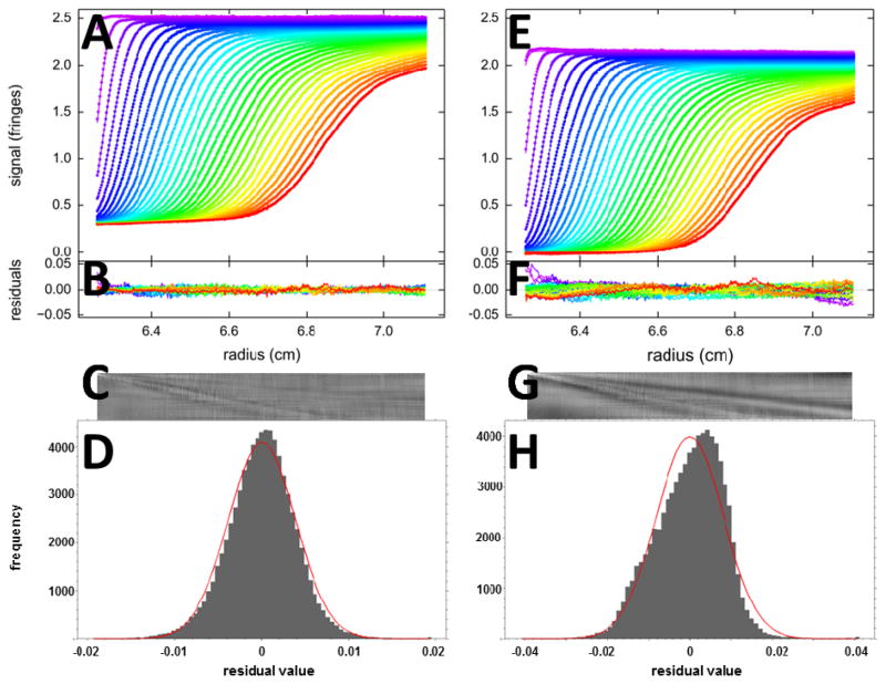
Figure 1.
Fits with two different models for SV data of BSA sedimenting at 50,000 rpm: (A – D) A c(s) analysis leads to a good fit with rmsd of 0.0039 fringes (Z-value 160); (E – H) a two discrete species model leads to an inadequate fit with rmsd of 0.0081 fringes (Z-value 224). The top panels (A, E) show the raw data (points, only every 2nd scan shown) and best-fit profiles (lines). Panels B and F are an overlay of the residuals, and C and G are the corresponding residual bitmaps (with time indicated by row number, and radius by column number of pixel). The residuals histogram is shown in panels D and H, with the grey bins indicating the frequency of residuals of a certain magnitude, and the red solid line the ideally expected distribution of residuals for normally distributed noise with the same rmsd, leading the H-numbers of 0.6% and 3.2%, respectively.

