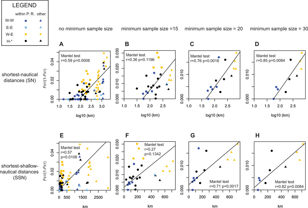
Figure 4. Pair-wise genetic distances in function of pair-wise geographical distances.
The first, second, third and fourth columns (left- right) show the plots of genetic versus geographic distances when the analysis include all localities (n=14), only localities with >=15 genotypes (n=8), >=20 genotypes (n=6) and >=30 genotypes (n=5). The top (A to D) and bottom rows (E to H) respectively show the plots for shortest-nautical (SN) and shortest-shallow-nautical (SSN) geographic distance. SN values were log10 transformed due to the bi-dimensionality of the model assumed. In all cases, FST(1-FST) between pair-wise served as a genetic distances. For each plot, RMA regressions were drawn with black lines. Results of the Mantel tests realized in each case were directly appended on the graphs. W-W: comparisons between two localities from the Western region. E-E: comparisons between two localities from the Eastern region. W-E: comparisons between one Western locality and one Eastern locality. H-*: comparisons between one hybrid locality and any other locality. The region of origin of each locality was determined using Structure results (Figure 3).

