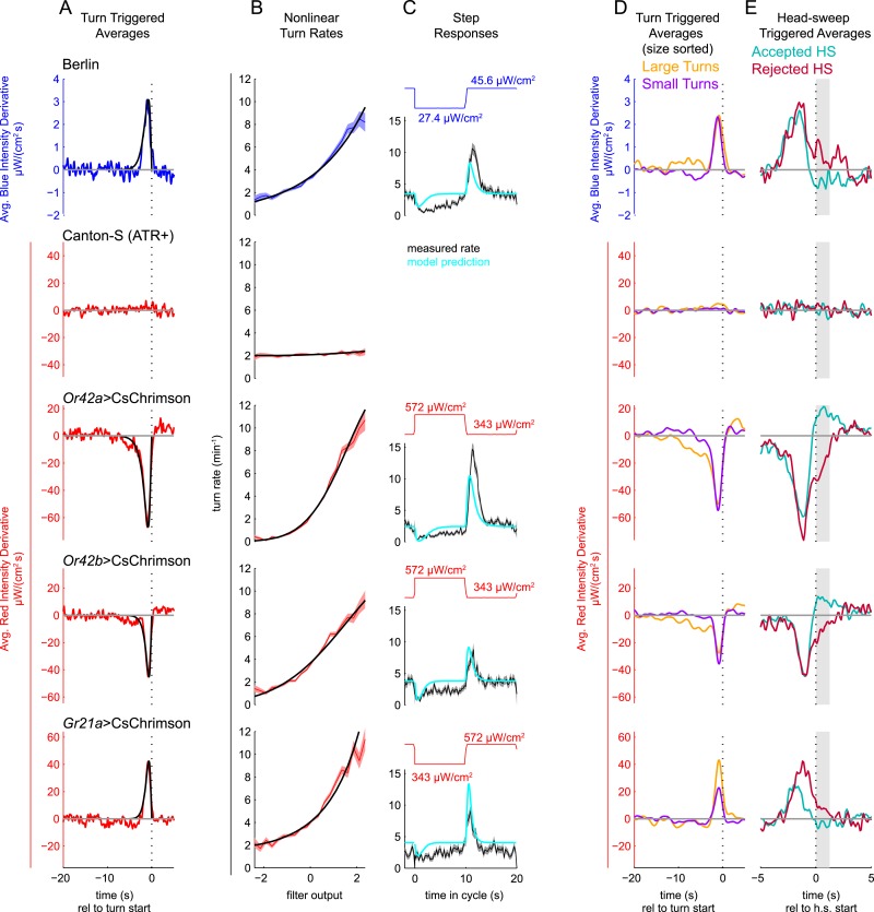
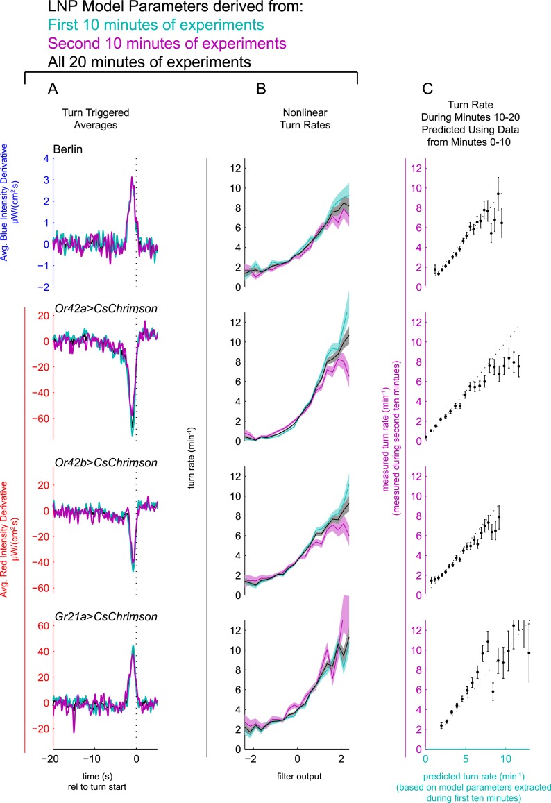
Figure 2. Unimodal reverse-correlation experiments.

Top row, Berlin wild-type larvae were stimulated with blue (λ_peak = 448 nm; max intensity = 74 μW/cm²) light. All other rows, larvae of indicated genotype were stimulated with red light (λ_peak = 655 nm; max intensity = 911 μW/cm²) while constant dim blue light (intensity = 3.7 μW/cm²) served as a visual mask. Column A: Turn triggered average. Average stimulus preceding (and following) each turn initiation. Turns are initiated at time 0 (indicated with dashed line). The black line is the smoothed TTA used as the linear filter. Column B: Measured turn rates as a function of calculated filter output. Line and shaded region represent mean turn rate and standard error due to counting statistics. Black line is the nonlinear turn rate modeled as a ratio-of-Gaussians (Pillow and Simoncelli, 2006). Column C: Step responses predicted by LNP model. Square waves of light with period 20 s and duty cycle 50% were presented to larvae. The LNP model was used to predict the resulting turn rates. Top graphs: light level vs time in cycle. A favorable change happens at t = 0 and an unfavorable change at t = 10 s. Bottom graphs: measured and predicted turn rates vs time in cycle. Black line and shaded region represent mean turn rate and standard error due to counting statistics. The cyan line is the exact prediction of the model using the parameters found from the corresponding reverse-correlation experiments. (A, B) The stimulus and analysis were cyclic, so the time range from −2 to 0 s is identical to that from 18–20 s. Column D: Size-sorted turn-triggered average. As in A, but turns were sorted into large (heading change during turn > rms heading change) and small turns. Displayed averages are lowpassed with a Gaussian filter (σ = 0.5 s) to clarify the long time-scale features. Column E: Head-sweep triggered average (for first head-sweep of turn). Average stimulus surrounding accepted (teal) and rejected (red) head-sweeps. Head sweeps were initiated at time t = 0 and concluded at a variable time in the future. The mean head-sweep duration (1.25 s) is indicated by the shaded region. See Table 1 for number of experiments, animals, and so on.

DOI: http://dx.doi.org/10.7554/eLife.06229.004

Figure 2—figure supplement 1. LNP model parameters are stable for duration of 20 min experiments.

Experiments of Figure 2 analyzed separately using data only from the first 10 min of experiment (teal) or only from the second 10 min of experiment (purple) or from entire 20 min data set (black). Column A: Turn triggered average. As in Figure 2A. The same convolution kernel is recovered from all three data sets. Column B: Measured turn-rates as a function of calculated filter output. As in Figure 2B. The turn rates vary across the three data sets mainly at high values of the filter output (stimulus conditions most likely to lead to turning). Column C: LNP model fits can predict response to white noise signals. Data from the first 10 min of the experiments were used to find LNP model parameters. The parameterized models were then used to predict the turn rate at each time point during the second 10 min of experiments. The measured turn rate during the second 10 min is plotted as a function of the model predictions. At high turn rates, for visual and fictive attractive odor stimuli, the turn rate is lower in the final 10 min than predicted by fits to the first 10 min, suggesting modest adaptation. For fictive CO₂, the measured turn rate is higher than predicted, suggesting modest sensitization. Error bars represent the uncertainty due to counting statistics.

DOI: http://dx.doi.org/10.7554/eLife.06229.005