FIG. 2.

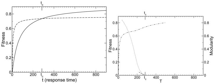
Shown is the fitness of an evolving system. a) The fitness of the non-modular (〈g₀〉, solid) and block-diagonal (〈g₁〉, dashed) system are shown, starting from a random initial configuration. These 〈g₀〉 and 〈g₁〉 are inputs to the theory. The modular system is taken to be more fit at short time and less fit at long time. b) The evolved, steady-state fitness of a system predicted by the theory in a changing environment (dot dashed), shown for varying T and p = 1. The fitness follows the high-modularity curve at rapid environmental changes, small T, and the low-modularity curve at slow environmental changes, large T. Since p = 1, the function f_p=1,T (M) = 〈g(M)〉(t = T). The function 〈g(M)〉 is here taken for simplicity to be (1−M)〈g₀〉(t)+M〈g₁〉(t). Note the modularity tends to 1 and the fitness to 〈g₁〉 for rapid environmental change (small T), and the modularity tends to 0 and the fitness to 〈g₀〉 for slow environmental change (large T). The modularity calculated from theory, Eq. (13), is shown (dotted). Also shown is the theoretical result for small M, Eq. (15), to first order in l/L (short dashed). In this example L = 120, l = 10, μ = 0.01, and C = 5.77. For these particular 〈g₀〉 and 〈g₁〉, the modularity emerges only for environmental changes that occur on a timescale T < t_c ≈ 285.