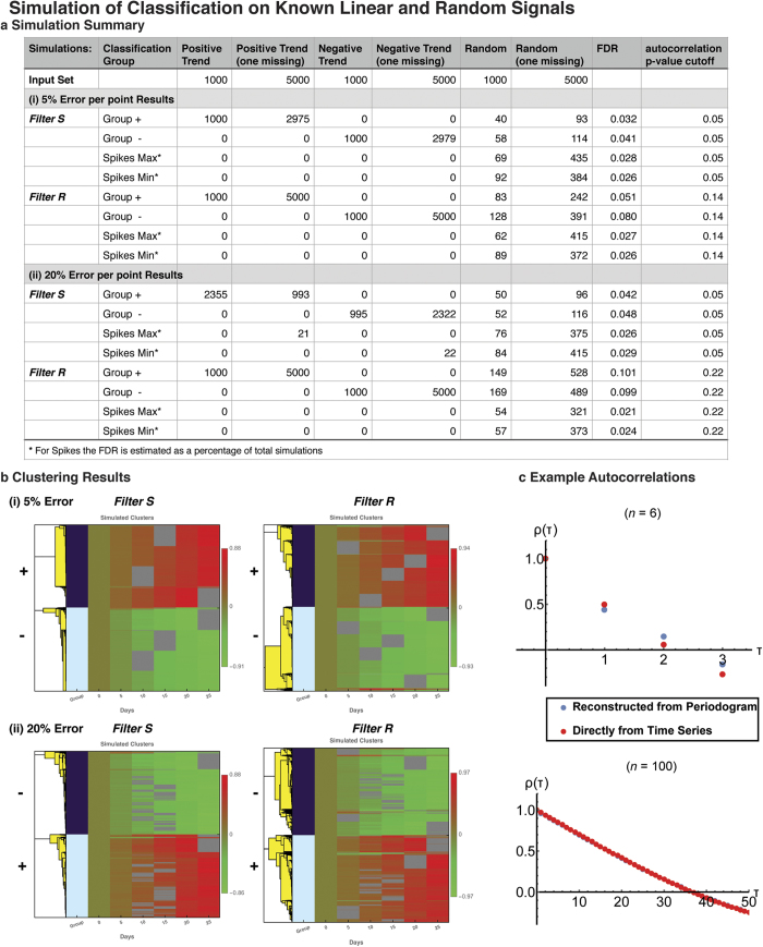
Figure 2. Simulation of Random Time Series.

(a) Simulations of the autocorrelation classification methodology were performed to assess robustness and reconstruction of temporal trends in known linear signals. The example illustrates a random realization that corresponds to a simulation of: 12,000 linear signals, of equal numbers of positive (+) or negative slope/trend (−), combined with a randomly generated equivalent set of 6000 random signals, and in randomized order. The numbers in each set were equally distributed between having zero or one time point missing (excluding the first one which is used as a reference). Additionally a simulation of 100,000 random signals was used as a background of bootstrap simulation. In particular, for simulations of linear signals with 5% random error per timepoint, Filter S corresponds to a strict p < 0.05 cutoff for autocorrelation at lag 1 (random series bootstrap, n = 100,000). In Filter R the p-value is relaxed until the entire set of linear trends is recovered. As seen, this results in modest false discovery rates. The simulation was repeated for linear signals with 20% error per timepoint for both filters. The corresponding heatmaps and clustering are shown in (b). (c) The reconstruction of autocorrelations from the periodogram, and the exact autocorrelations are shown for a straight signal, for a series of n = 6 and n = 100 time points. For n = 100 the reconstruction is indistinguishable from the exact calculation in the figure.