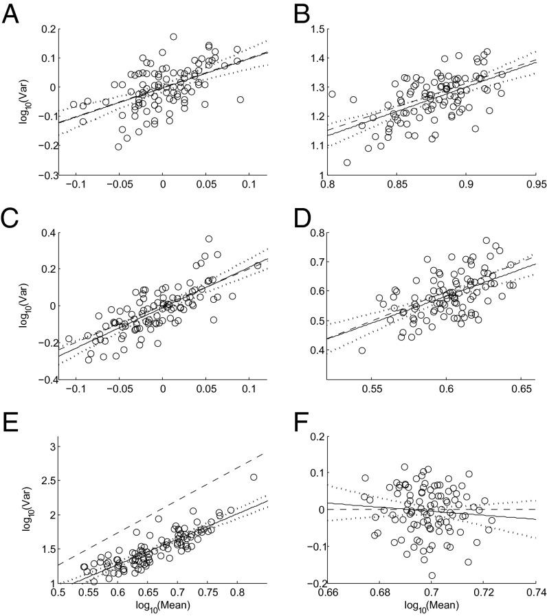
Fig. 1.

Taylor’s law with positive slope arises from random samples from a single (A) Poisson (λ = 1), (B) negative binomial (r = 5, p = 0.4), (C) exponential (λ = 1), (D) gamma (α = 4, β = 1), and (E) lognormal (µ = 1, σ = 1) distribution, but not from a (F) shifted normal [5 + $\mathcal{N}$(0,1)] distribution [i.e., a $\mathcal{N}$(0,1) distribution with 5 added to each value to make each block’s mean positive with high probability]. For each panel, 10,000 iid observations from the selected distribution were arranged randomly in a square matrix with n = 100 rows and N = 100 columns. For each column j, the sample mean m_j and the sample variance v_j were calculated and plotted on log-log coordinates using open circles, j = 1, …, N. The solid black line is the least-squares linear regression log₁₀ v_j = log₁₀ a + b log₁₀ m_j. The dotted curved lines above and below the solid black line give the 95% confidence interval of the regression line. Slope and intercept of the dashed black line were computed analytically from Eqs. 3 and 4, respectively (Table 1), using the population moments used to generate the observations, not the sample moments of the observations. Population skewness in each distribution is 1 (Poisson), 0.9238 (negative binomial), 2 (exponential), 1 (gamma), 6.1849 (lognormal), and 0 (shifted normal).