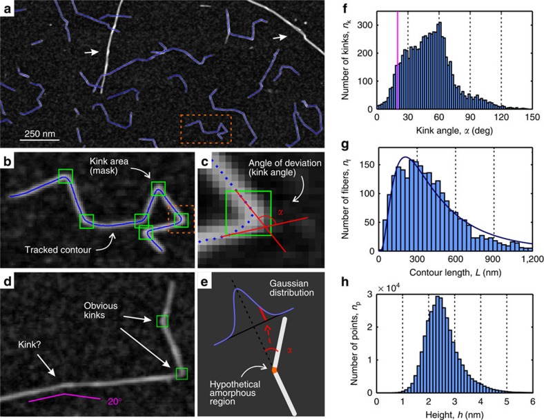
Figure 4. Tracking procedure of W-CNF and results of statistical analysis on fibril contours.

(a) AFM image with tracked contours (blue curves). Objects that are considered to be bundles of CNF were discarded from tracking (examples are pointed by white arrows). (b) Magnified region of the AFM image from a containing one tracked contour. The green frames are special masks, placed manually, allowing tracking of the contours with heterogeneous flexibility. In the statistical analysis these areas were considered to represent the vicinities of kinks. (c) Magnified region of the AFM image from b showing the particular mask area with the contour represented by its points. Two segments of the contour that enter or exit the kink area define an angle of contour deviation (kink angle) α. (d) Example of CNF with two obvious kinks and one uncertain case. It is non-trivial to state whether this is a kink or elastic bending due to thermal fluctuations. An example of the 20° angle is shown as a guide to eye. (e) The kink angle distribution should have a Gaussian shape in case of hypothetical amorphous regions corresponding to kinks because of equal probability to bend in both directions. (f) Kink angle distribution of 2,380 tracked CNFs. The bins in the region below 20° (violet line corresponds to this cutoff value) can lack some counts because of the manual threshold of kink angle assignments. (g) Contour length distribution fitted with normalized density function of the log-normal distribution with parameters μ=5.94 and σ=0.77. (h) Height distribution of all points along all tracked contours. The most probable height value is 2.35 nm.