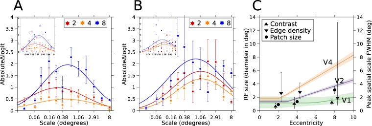
Figure 4.

Coefficients for RMS contrast and edge density across scale, and interpreted as receptive field size. (A) Absolute change in the linear predictor for RMS contrast changes across spatial scales, for three eccentricities. The abscissa shows the standard deviation of the Gaussian-weighted scale in degrees of visual angle. The ordinate shows the absolute value of the change in the logit (linear predictor) from the 16th percentile of RMS contrast at that scale to the 84th percentile, holding patch size at its threshold value for that eccentricity (Figure 3) and all other predictors in the model at their mean value. This can be thought of as a normalized absolute regression coefficient. Curves show the best fitting Gaussian function for each eccentricity (functions were fitted to all observers' data rather than means, but points show mean values between observers to aid visibility). Error bars show the SEM between the three observers. The inset Figure shows the data for individual observers from (A). Colors code eccentricity as in A. Different observers are displayed with different markers (TW = circle, PB = square, and N1 = diamond) and Δ logits whose signed value is positive are shown as solid markers, negative Δ logits as open markers. (B) Same as (A) for edge density. (C) Inferring receptive field sizes from model outputs. Hinged lines show changes in receptive field diameter as eccentricity increases for three visual areas V1, V2, and V4 in non-human primates (parameters kindly provided by J. Freeman). The shaded regions around the hinged line fits show 95% confidence regions estimated from the parameter uncertainties provided by J. Freeman. Triangles pointing up show the full width at half maximum of a Gaussian with a standard deviation given by the peak of Gaussian fits in (A), for RMS contrast. Down-pointing triangles show the same for edge density, from (B). Error bars on these data points show 95% confidence intervals derived from fitting to data in (A) and (B) sampled with replacement 4999 times. Circles plot the average threshold patch diameter in degrees (Figure 3) and error bars show +/- 1 standard deviation between observers (error bars at 2 and 4 degrees are smaller than the marker). In good agreement with Bouma's law, threshold patch size estimates are consistent with the sizes of receptive fields in area V2 of primate brains. RMS contrast peaks are more consistent with V1 receptive fields, and edge density is more consistent with extra striate regions (albeit with much greater uncertainty).