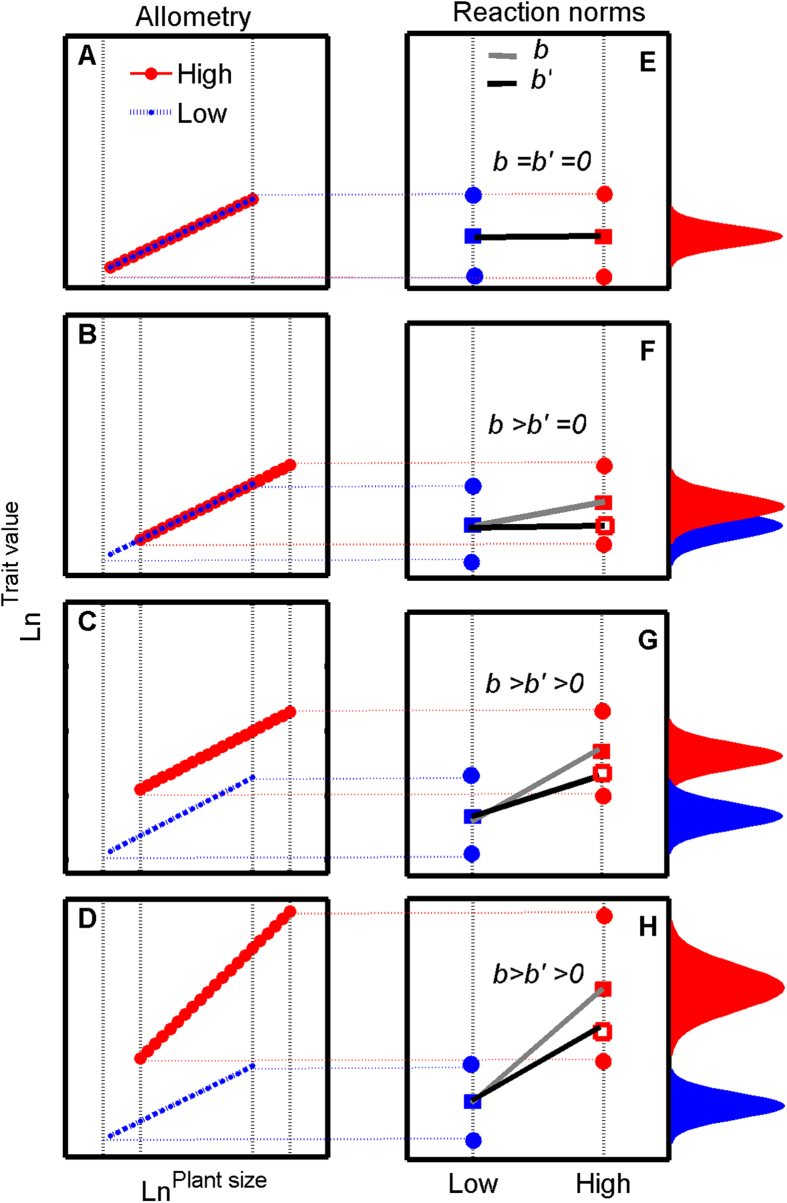
Figure 2. Scenarios for re-evaluating the levels of phenotypic plasticity.

(A) Lines overlap (no phenotypic plasticity); (B) lines share a common slope and also share a common elevation, but shift in location along the common slope (apparent plasticity); (C) lines share a common slope but difference in elevations (apparent plasticity + true plasticity); and (D) the slopes are not equal (apparent plasticity + true plasticity). In an allometric view, different slopes and/or different elevations show that the biomass allocation is affected by varying environment factors (true plasticity). However, the allometric relationships among traits are universal in plants, thereby the phenotypic plasticity in C and D also include the apparent plasticity. The blue (or red) dots in (E) represent the trait at sample start time, t_s and sample end time, t_e under a low-resourc_e environment, e₁ (or high-resource environment, e₂), respectively. The blue (or red) squares represent the phenotypes in sample time, t. The empty blue (or empty red) squares represent the phenotypes in sample of the same plant size. The right curves represent the normal distribution of trait value in a low-resource (blue) and a high-resource (red) environment, respectively. The representation is the same for (F–H).