Fig. 3.
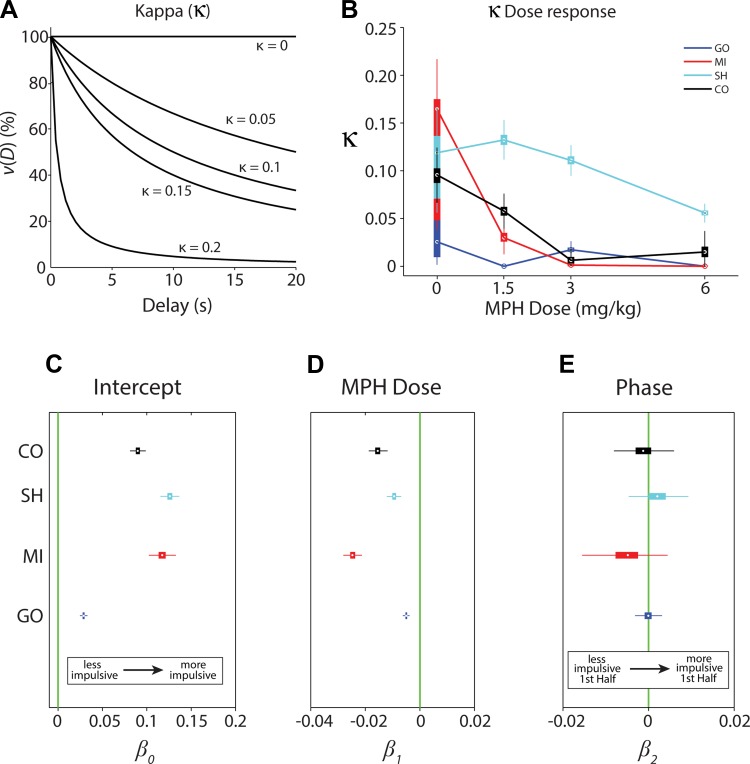
Analysis of discounting constant (κ). A: examples of hyperbolic discounting functions for simulated values of κ. Discounted value of the LL [ν(D)] plotted as a function of LL delay (in s). As κ increases, the discounting function becomes steeper, and the LL loses more value with time, indicating greater impulsivity. B: discounting constant (κ) plotted as a function of MPH dose (mg/kg) for all 4 subjects. Data are presented as box plots for each subject at each dose. Points represent the median values of bootstrapped data; boxes represent 25th and 75th percentiles; whiskers extend to the 99th percentile. C–E: general linear model (GLM) parameter estimates for κ. Data are presented as box plots. Points represent the median estimates of bootstrapped data; boxes represent 25th and 75th percentiles; whiskers extend to the 99th percentile. C: estimate of intercept (β0subject) for the discounting constant, κ. Intercept values indicate subject's average κ value over conditions. D: estimate of slope of MPH dose effect (β1subject) on κ. Slope values indicate the linear trend resulting from varying doses of MPH treatment. E: estimate of the phase effect (β2subject), testing for a difference in κ between the 1st and 2nd half of the session. Values >0 would indicate a larger κ in the 1st compared with the 2nd half of the session.

