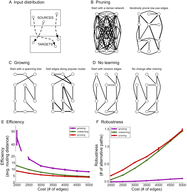
Fig 3. Computational network model and comparison between pruning and growing.

(A) Example distribution (2-patch) for source-target pairs. (B) The pruning algorithm starts with an exuberant number of connections. Edges commonly used to route source-target messages are retained, whereas low-use edges are iteratively pruned. (C) The growing algorithm begins with a spanning-tree and adds local shortcut edges along common source-target routes. (D) The no-learning algorithm chooses random edges and does not attempt to learn connections based on the training data. (E+F) Learned networks were evaluated by computing efficiency (E, the average shortest-path distance amongst test pairs) and robustness (F, the average number of short alternative paths between a test source and target). Error bars indicate standard deviation over 3 simulation runs.