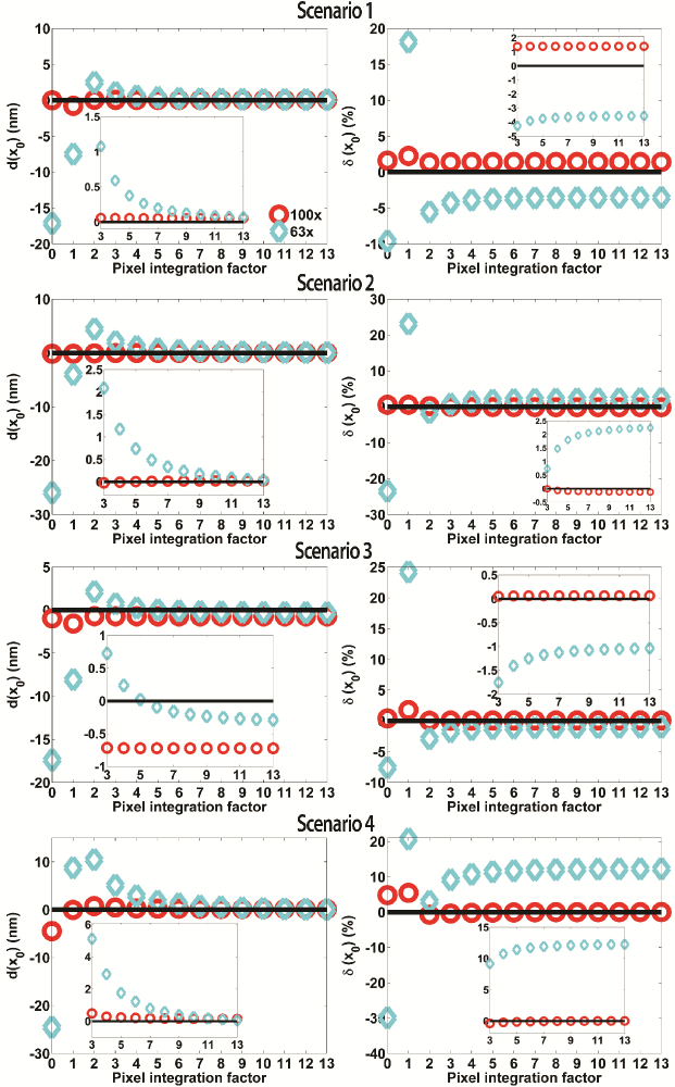
Fig. 3.

2D Gaussian profile results: difference d(x₀) between the median of the x₀ estimates and the true value x₀ (left-hand side plots), and percentage difference δ (x₀) between the standard deviation (with respect to the median) of the x₀ estimates and the PLAM for x₀ (right-hand side plots), as functions of the PIF used to integrate the image profile during estimation. For each scenario of Table 1, results are shown for a 63× (cyan⋄) and a 100× (red○) data set, simulated at PIF = 13 using the 2D Gaussian profile with parameters given in Section 4. Each data set is fitted with a 2D Gaussian profile by an ML estimator, with PIF values ranging from 0 to 13. In all plots the horizontal line denotes 0, and the inset shows the results for PIF ≥ 3.